Chapter 6: Vector Search
What Is It?
A vector index stores high-dimensional numerical representations of data and answers a different kind of question from the ones we’ve asked so far. Not “find items where this field equals that value” but “find items that are most similar to this one.” Similarity is measured by distance in vector space – items whose vectors are close together are considered similar, regardless of whether they share any explicit property values.
Neo4j supports native vector indexes with approximate nearest neighbor (ANN) search, enabling fast similarity queries directly in Cypher. You create the index on a list property that holds the vector, call db.index.vector.queryNodes() to retrieve the k nearest neighbors, and compose the result with any further Cypher – graph traversal, property filters, aggregations – in the same statement.
The key word is approximate. ANN search trades a small amount of recall for a large gain in speed. For most real-world similarity use cases – find me items that look like this one, find documents semantically similar to this query – approximate results are indistinguishable from exact results in practice.
When Would You Reach for It?
Vector search earns its place when similarity is the query rather than equality. Traditional indexes answer exact match and range queries. Vector indexes answer “nearest neighbors” queries, which is the right abstraction for image similarity, semantic text search, recommendation and anomaly detection.
Reach for Neo4j’s vector search when:
- You want to find items similar to a given item, where “similar” means close in a learned or computed embedding space
- You’re already using Neo4j and want to combine vector similarity with graph traversal in a single query
- You need to filter similarity results by graph structure – “find the 5 most similar items that belong to this category”
The last point is where Neo4j’s vector search stands out. A standalone vector database returns similar vectors. Neo4j can return similar vectors that also satisfy a graph pattern – traversing relationships to restrict the search space or enrich the results. That combination is what we demonstrate in this chapter and it’s what chapter 7 builds on directly.
The Use Case
For this chapter we’ll build a clothing image similarity explorer using the Zalando Fashion-MNIST dataset – 70,000 labeled grayscale images across 10 clothing categories, released under the MIT License. We store each image as a 784-element vector (the flattened, normalized pixel values) alongside a graph that connects each item to its category. Users can pick a random item from any category, run a k-nearest-neighbor search against the full 70,000-item index and see which images are most visually similar.
The Data
Fashion-MNIST contains 60,000 training images and 10,000 test images across 10 clothing categories: t-shirt/top, trouser, pullover, dress, coat, sandal, shirt, sneaker, bag and ankle boot. Each image is 28x28 pixels in grayscale.
The vector representation is straightforward – no embedding model required. We normalize pixel values to [0,1] and flatten each 28x28 image into a 784-element float vector. This is a deliberate choice: pixel vectors are interpretable, require no external model and are sufficient to demonstrate the mechanics of vector search and graph-filtered similarity.
The graph model is:
(:Item {uid, id, label, split, vector})-[:BELONGS_TO]->(:Category {name})
id is the zero-based index within the split (0-59999 for train, 0-9999 for test). split is "train" or "test". uid is a globally unique string combining both – "train_0", "test_500" – and is the uniqueness key. Two items can share the same id if they’re in different splits. vector holds the 784-element list property that the vector index is built on.
Figure 6-1 shows one example from each of the ten clothing categories.
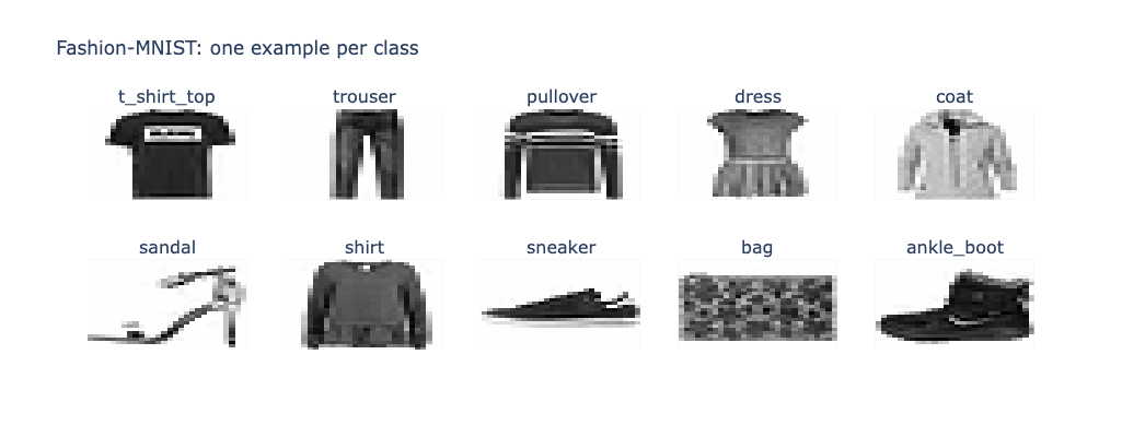
Figure 6-1. Fashion-MNIST Examples.
Building the Application
Prerequisites
You’ll need a Neo4j Aura free-tier instance with the connection details stored as environment variables.
Fashion-MNIST is fetched automatically via scikit-learn’s fetch_openml.
Loading the Data
We fetch Fashion-MNIST via scikit-learn, normalize and flatten the images, then build two DataFrames:
fashion = fetch_openml(name="Fashion-MNIST", version=1, as_frame=False)
X, y = fashion.data, fashion.target.astype(np.uint8)

train_images_raw = X[:60000].reshape(-1, 28, 28)
test_images_raw  = X[60000:].reshape(-1, 28, 28)

# Normalize to [0, 1] and flatten to 784-element vectors
train_images = (train_images_raw.astype("float32") / 255.0).reshape(-1, 784)
test_images  = (test_images_raw.astype("float32")  / 255.0).reshape(-1, 784)

train_df = pd.DataFrame({
    "id":     np.arange(len(train_images)),
    "vector": list(train_images),
    "label":  [CLASSES[l] for l in train_labels],
    "split":  "train"
})
Loading the Graph
We clear the database, create uniqueness constraints, load Category nodes for the 10 classes, then load Item nodes in batches of 500:
session.run("""
    CREATE CONSTRAINT category_name IF NOT EXISTS
    FOR (c:Category) REQUIRE c.name IS UNIQUE
""")
session.run("""
    CREATE CONSTRAINT item_uid IF NOT EXISTS
    FOR (i:Item) REQUIRE i.uid IS UNIQUE
""")

session.run("""
    UNWIND $names AS name
    MERGE (:Category {name: name})
""", names=CLASSES)
The uniqueness constraint is on uid, not id. Without it, items from different splits with the same integer id would conflict. The uid field – "train_0", "test_500" – is unique across the entire graph.
Items are loaded in chunks of 500 using UNWIND. Each item is linked to its category via BELONGS_TO:
session.run("""
    UNWIND $rows AS row
    CREATE (i:Item {
        uid:    row.uid,
        id:     row.id,
        label:  row.label,
        split:  row.split,
        vector: row.vector
    })
    WITH i, row
    MATCH (c:Category {name: row.label})
    CREATE (i)-[:BELONGS_TO]->(c)
""", rows=chunk)
With 70,000 items batched at 500, this is 140 transactions. Expect the full load to take several minutes on Aura’s free tier.
Creating the Vector Index
A single Cypher call creates the vector index using Euclidean distance:
session.run("""
    CREATE VECTOR INDEX item_vector IF NOT EXISTS
    FOR (i:Item) ON (i.vector)
    OPTIONS {indexConfig: {
        `vector.dimensions`: 784,
        `vector.similarity_function`: 'euclidean'
    }}
""")
Euclidean distance is appropriate for pixel vectors – it measures the total intensity difference across all 784 pixels. For semantic text embeddings, cosine similarity is usually the better choice.
t-SNE Visualization
Before querying the index, we use t-SNE to project the 784-dimensional vectors into 2D and verify that the categories form distinct clusters. We sample 60,000 training items and run t-SNE with the Barnes-Hut algorithm:
tsne = TSNE(
    n_components=2,
    random_state=42,
    method="barnes_hut",
    perplexity=30,
    max_iter=1000
)
X_tsne = tsne.fit_transform(train_images[:60000])
The resulting scatter plot, colored by class, shows clear clusters for most categories – trousers and bags are well separated; t-shirts, shirts and pullovers cluster more closely, which matches the visual similarity of those garments. This gives us confidence that the vector index will return meaningful nearest neighbors.
Figure 6-2 shows the result – most categories form distinct clusters, though t-shirt, shirt and pullover overlap, which matches their visual similarity.
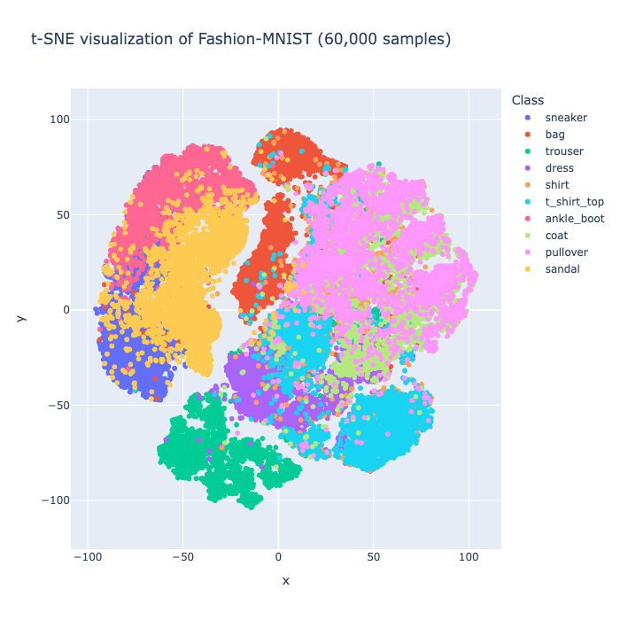
Figure 6-2. t-SNE Projection.
Query 1: k-NN Within the Training Set
The standard k-NN query fetches the query vector from Neo4j, then calls the vector index:
# Fetch the query vector
q = session.run("""
    MATCH (i:Item {id: $id, split: $split})
    RETURN i.vector AS vector, i.label AS label
""", id=QUERY_ID, split="train").single()

# k-NN search
result = session.run("""
    CALL db.index.vector.queryNodes('item_vector', $k, $vector)
    YIELD node AS i, score
    WHERE i.split = $split
    RETURN i.id AS id, i.label AS label, i.split AS split, score
    ORDER BY score DESC
""", k=K * 3, vector=q["vector"], split="train")
Two things to note. First, the score from Euclidean distance is inverted – a higher score means greater similarity (closer in vector space), not greater distance. Second, we fetch k * 3 candidates and filter to k after excluding the query item itself, which always appears in the results with a perfect score.
The image grid renders the query item and its nearest neighbors using Plotly’s go.Heatmap with colorscale="gray_r" – inverted grayscale gives white backgrounds with dark clothing outlines, which reads more naturally than the raw dark-background representation.
Query 2: k-NN Within the Test Set
The same pattern applied to a test-split query item. Because train and test items are in the same index, we filter by i.split = 'test' in the WHERE clause.
Query 3: Cross-Set Similarity Search
A train item queries against the test set, or vice versa. This tests whether the vector representations generalize across splits – whether a training image of a dress finds similar test images of dresses:
result = session.run("""
    CALL db.index.vector.queryNodes('item_vector', $k, $vector)
    YIELD node AS i, score
    WHERE i.split = 'test'
    RETURN i.id AS id, i.label AS label, i.split AS split, score
    ORDER BY score DESC
""", k=K * 3, vector=query_vector)
For most query items, the top test-set neighbors are in the same category as the query – the pixel vectors are consistent enough across the train/test split that cross-set search works reliably.
Query 4: Graph-Filtered k-NN
This is where the graph model adds value. We restrict the search to a specific category by traversing the BELONGS_TO relationship after the vector index call:
result = session.run("""
    CALL db.index.vector.queryNodes('item_vector', $k, $vector)
    YIELD node AS i, score
    MATCH (i)-[:BELONGS_TO]->(c:Category {name: $category})
    RETURN i.id AS id, i.label AS label, i.split AS split, score
    ORDER BY score DESC
""", k=K * 10, vector=query_vector, category="dress")
We fetch k * 10 candidates to ensure enough remain after the category filter. This is a post-filter pattern – the vector index finds the approximate nearest neighbors globally, then the graph traversal filters to the target category. For a balanced dataset like Fashion-MNIST, fetching 10x candidates is sufficient. For unbalanced categories a larger multiplier may be needed.
This pattern – vector search then graph filter – is the foundation of what chapter 7 builds into a full fraud detection system.
The Streamlit App
The app has a sidebar with controls for the query category, query split, results split filter, results category filter and k. A “Pick random item and search” button selects a random item from the chosen category and split, fetches its vector from Neo4j and runs the k-NN search.
The main area shows a summary of the query item and result count, an image grid of the query item and its nearest neighbors rendered as Plotly heatmaps, and a category breakdown bar chart showing which categories appear in the results. The image grid renders both the query image and result images from the in-memory Fashion-MNIST arrays rather than fetching pixel data from Neo4j – the vectors stored in Neo4j are the normalized float versions, not the original uint8 values needed for display.
Results persist in st.session_state across re-runs so the display doesn’t disappear when sidebar controls are adjusted.
What You’d Hit in Production
ANN vs exact search. Neo4j’s vector index uses approximate nearest neighbor search. For the Fashion-MNIST use case the approximation is excellent – the top-k results are indistinguishable from exact results in practice. For use cases where recall must be guaranteed (medical imaging, legal document retrieval), exact search may be required, which is slower but available.
Index creation time. Creating the vector index over 70,000 items with 784 dimensions takes a few minutes on Aura’s free tier. The index creation is asynchronous – check the index state before querying.
Post-filter overhead. The graph-filtered k-NN query (Query 4) fetches k * 10 candidates to ensure enough survive the category filter. If the target category is rare in the index, you may need a larger multiplier. An alternative is pre-filtering – restricting the index scan to nodes of the target category – but this isn’t supported in Neo4j’s current vector index implementation.
Vector storage. Each 784-element float32 vector takes around 3KB of storage. 70,000 vectors takes around 200MB, which is within Aura’s free-tier limit but leaves little headroom. For higher-dimensional vectors – 384-element sentence embeddings, 1536-element OpenAI embeddings – storage requirements grow accordingly.
The split filter. The WHERE i.split = $split clause in queries 1 and 2 runs after the ANN index returns candidates. It’s a post-filter, not a pre-filter. For very unbalanced splits, fetch more candidates than you need.
Going Further
Vector search finds similar items by distance in vector space. Graph traversal finds connected items by relationship. In this chapter we combined them: a vector search followed by a graph filter in a single Cypher statement. That combination is powerful, but both steps still ran independently – the vector search found candidates globally, then the graph reduced them.
Chapter 7 inverts the order and tightens the integration. We use vector search to find semantically suspicious transactions, then use graph traversal to confirm whether those transactions form a circular money flow – a fraud ring. The vector component identifies candidates the graph component couldn’t find alone; the graph component validates structure the vector component can’t see. That’s the full combination, and it’s where this book ends up.