Welcome
How to Cite This Book
If you use this book in your work, please cite it as:
APA: Chaudhri, A. (2026). Neo4j Beyond the Graph. Self-published. https://beyond-the-graph.github.io/
BibTeX:
@online{chaudhri2026beyondthegraph,
  author  = {Chaudhri, Akmal},
  title   = {Neo4j Beyond the Graph},
  year    = {2026},
  url     = {https://beyond-the-graph.github.io/},
  urldate = {2026-09-24}
}
Cover
License
Copyright
Copyright © 2026 Akmal Chaudhri. All rights reserved.
Publication Information
First published: September 2026
The latest version of this book, together with updates, errata and additional resources, is available at:
Book License
Neo4j Beyond the Graph is licensed under the Creative Commons Attribution-NonCommercial-NoDerivatives 4.0 International License (CC BY-NC-ND 4.0).
You are free to copy and redistribute this book in any medium or format under the following conditions:
- Attribution - You must give appropriate credit, provide a link to the license and indicate if changes were made.
- NonCommercial - You may not use the material for commercial purposes.
- NoDerivatives - If you remix, transform or build upon the material, you may not distribute the modified material.
The full license text is available at:
creativecommons.org/licenses/by-nc-nd/4.0
Code License
Unless otherwise stated, all code samples, notebooks, scripts and source files accompanying this book are licensed under the Apache License 2.0.
You are free to use, modify and redistribute this code, including for commercial purposes, subject to the terms of the Apache License 2.0.
The full license text is available at:
apache.org/licenses/LICENSE-2.0
This distinction means that the book’s written content is protected under the Creative Commons license, while the accompanying code remains freely available for use, modification and integration into your own projects.
Trademarks
Product names, company names and logos mentioned in this book may be trademarks or registered trademarks of their respective owners.
Their inclusion is for identification and educational purposes only and does not imply any affiliation with, sponsorship by or endorsement from the respective trademark holders. All trademarks remain the property of their respective owners.
Disclaimer
The information in this book, including all code samples, scripts and notebooks, is provided “as is” without warranty of any kind, express or implied.
The author makes no representations or warranties regarding the accuracy, completeness, reliability or suitability of the information contained herein for any particular purpose.
Examples are provided solely to illustrate technical concepts, database patterns and software architectures.
Readers are responsible for independently validating all code, configurations and recommendations before using them in production environments.
To the fullest extent permitted by law, the author shall not be liable for any direct, indirect, incidental, special, consequential or other damages arising from the use of or inability to use, the information, code or techniques described in this book.
About the Author
Akmal Chaudhri is a technical leader, educator and author with extensive experience in databases, AI and developer relations. He specializes in technical writing, developer education and community building, helping engineers and organizations understand and adopt complex technologies through clear, practical and engaging content. He is a frequent international speaker, a published author and a contributor to industry discussions on data platforms, AI and software development.
Today, Akmal works in developer education at Neo4j, where he focuses on technical content, workshops and community initiatives. While his professional role has evolved, this book represents an independent exploration of Neo4j.
Based in the United Kingdom, Akmal continues to work at the intersection of databases, AI and developer tooling, helping developers build modern data-driven applications.
For book updates, code samples and additional resources, visit the Book website.
To connect professionally or follow his latest work, visit LinkedIn.
Introduction
Neo4j Beyond the Graph
Ask a developer what Neo4j is and you’ll almost always get the same answer: a graph database. That answer is correct, but it’s also incomplete, and the gap between what most people know about Neo4j and what Neo4j can actually do is the reason this book exists.
Neo4j started as a graph database and graph traversal remains its core strength. If you need to find the shortest path between two nodes, detect communities in a network or traverse a hierarchy in milliseconds, nothing beats native graph storage. But over the years Neo4j has grown into something considerably broader. It now supports full-text search, native geospatial queries, temporal reasoning, document-style properties, vector similarity search and the combination of graph traversal with vector search that makes it genuinely unique in the database landscape. These aren’t bolt-on features or integrations with external systems. They’re built in and they work together.
Many Neo4j users don’t know this. They connect to an Aura instance, model their domain as nodes and relationships, write some Cypher and move on. That’s a perfectly valid use of the product. But it’s a fraction of what’s available and the chapters that follow are an attempt to close that gap.
What This Book Is About
Each chapter focuses on one Neo4j capability and one use case chosen to showcase it. We start with the native graph model – the foundation everything else builds on – and work outward from there. By the end you’ll have seen Neo4j handle transport networks, research literature, air quality data, financial time series, library inventories, image similarity and fraud detection, each using a different capability or combination of capabilities.
The progression is deliberate. We begin with what Neo4j is best known for and add capabilities one at a time, so each chapter extends your mental model rather than replacing it. By chapter 7, when we combine graph traversal with vector search to detect fraud rings, you’ll be drawing on everything that came before.
| Chapter | Capability | Use Case |
|---|---|---|
| 1 | Native Graph | London Underground routing |
| 2 | Full-Text Search | Research paper discovery |
| 3 | Geospatial | Air quality along the Pyrenees corridor |
| 4 | Temporal | S&P 500 stock price analysis |
| 5 | Document-Style Properties | Library inventory management |
| 6 | Vector Search | Fashion image similarity |
| 7 | Graph + Vector | Fraud ring detection |
Who This Book Is For
This book is written for developers and data engineers who already have some familiarity with Neo4j – you’ve run a Cypher query, you understand the node-relationship model – but haven’t explored the capabilities beyond the graph. It assumes you’re comfortable with Python and Jupyter notebooks. It doesn’t assume any prior experience with vector search, geospatial indexing or full-text search engines.
If you’ve been using Neo4j as a graph database and wondering what else it can do, this book is for you. If you’re evaluating Neo4j for a use case that isn’t purely graph-shaped – a search problem, a geospatial problem, a time series problem – this book is for you. If you’re building an application that needs several of these capabilities together, particularly the graph-plus-vector combination that closes the book, this book is for you.
How the Book Is Structured
Each chapter follows the same structure:
- What is it – a characterization of the capability, how it works inside Neo4j and what makes it distinctive
- When would you reach for it – the practical question answered upfront: when does this capability earn its place in your architecture?
- The use case – the specific scenario for that chapter, chosen because it genuinely fits the capability rather than to manufacture a demo
- The data – the dataset used and why it suits the problem
- Building the application – a hands-on walkthrough with code, including gotchas we encountered along the way
- What you’d hit in production – notes on limitations, operational considerations and scale
- Going further – what combining this capability with others unlocks and how it connects to later chapters
Every chapter comes with a Jupyter notebook and a Streamlit application. Chapter 3 is the exception, as the analysis notebook assumes the AQI data are already loaded, either by running the ingest notebook first or by importing the provided backup file.
A Note on the Dataset Choices
Some chapters use real-world data – London Underground station coordinates, Pyrenees air quality readings from IQAir, S&P 500 price history from Kaggle. Others use synthetic data generated in the notebook itself. In every case the choice was made to give the capability room to show what it can do: a transport network for graph traversal, tightly clustered financial amounts for fraud detection, high-dimensional pixel vectors for image similarity.
Where data comes from an external source it’s either publicly available under an open license or generated fresh by running the notebook. Two chapters require free-tier API keys: chapters 1 and 3 use CartoDB basemap tiles for Folium maps and chapter 3 additionally uses the IQAir API for air quality data. Both keys are available on free tiers at carto.com and iqair.com.
A Note on Aura
All examples in this book run against Neo4j Aura, the fully managed cloud service. Aura’s free tier provides enough storage and compute for every dataset in the book. The connection pattern is the same throughout: set four environment variables – NEO4J_URI, NEO4J_USERNAME, NEO4J_PASSWORD and NEO4J_DATABASE and every notebook connects without further configuration.
To follow along, you’ll need a free Aura account – sign up at Get Started for Free.
If you prefer to run Neo4j locally, everything works identically against Neo4j Desktop. The only adjustment is the connection URI and credentials.
Code and Notebooks
All notebooks, Streamlit applications and source code are available at:
Each notebook is self-contained and each Streamlit application has its own requirements.txt. A single combined requirements.txt at the repo root installs all Streamlit dependencies for all chapters at once – useful if you plan to work through the book from start to finish. You’ll need Python 3.12, a virtual environment and classic Jupyter installed locally.
Chapter 1: Native Graph
What Is It?
At its core, Neo4j stores data as nodes and relationships. A node represents an entity – a station, a person, a product. A relationship connects two nodes and carries a direction and a type – CONNECTS_TO, AUTHORED, PURCHASED. Both nodes and relationships can hold properties: a station has a name and coordinates, a connection has a line name.
This sounds simple, and it is. The power comes from what this model makes natural. In a relational database, finding connections between entities means writing joins – and the more hops you need to traverse, the more joins you write and the slower the query runs. In Neo4j, traversal is a first-class operation. Following a relationship from one node to another is a constant-time operation regardless of the size of the graph. A query that finds paths three, five or ten hops deep runs in the same fundamental way – following pointers through the storage engine – rather than computing a Cartesian product across tables.
Cypher, Neo4j’s query language, makes this traversal natural to express. A pattern like (a)-[:CONNECTS_TO*1..5]->(b) reads almost like English: find any path from a to b using CONNECTS_TO relationships, up to five hops deep. The same question in SQL requires a recursive CTE, a depth cap, careful deduplication and considerably more thought.
When Would You Reach for It?
The native graph model earns its place when the connections between entities are the point of the data, not a side effect of it. Transport networks are the textbook example: a station on its own is just a location, but the network of connections between stations is what makes it useful. Social graphs, supply chains, recommendation networks, knowledge graphs and fraud detection are all problems where the structure of the connections is the signal you’re trying to extract.
Reach for Neo4j’s graph model when:
- Your queries traverse multiple hops and the depth varies at runtime
- The relationships between entities carry meaning in their own right – type, direction, weight, timestamp
- You need shortest path, community detection or other graph algorithms as part of your application logic
- Joins in a relational model are becoming the performance bottleneck
A simple parent-child hierarchy or a single join doesn’t justify the switch. But as soon as you find yourself writing recursive CTEs or self-joins to answer questions about how entities connect, the graph model starts paying for itself.
The Use Case
For this chapter we’ll build a London Underground route explorer. Given any two stations, find the shortest path between them – the minimum number of stops and the sequence of line changes. Given a starting station, find all stations reachable within a given number of stops and visualize the spread of the network from that point. And surface a structural curiosity of the network: stations in the same fare zone that require surprisingly long journeys between them and stations in adjacent fare zones that are only one or two stops apart.
The Underground is a natural fit for the graph model. Stations are nodes. Connections between adjacent stations on the same line are relationships. The line name and color are properties on each relationship. The network topology – which station connects to which, and how – is exactly what the data are about.
The Data
We use three CSV files from the publicly available London Underground dataset:
london_stations.csv– stations with names, coordinates and zone informationlondon_connections.csv– direct connections between adjacent stationslondon_lines.csv– line names and hex color codes
Before loading, we merge line colors onto the connections and filter stations down to only those that appear in at least one connection. The graph we load into Neo4j has Station nodes and bidirectional CONNECTS_TO relationships between adjacent stations. Each station carries its name, latitude, longitude and zone. Each connection carries the line name and the line color.
One preprocessing detail: zone values in the raw data are sometimes composite strings like "3,4,5,6" for stations that straddle multiple zones. We keep these as-is on the node but filter them out when running zone-based analysis by matching only stations whose zone field is a single integer.
Building the Application
Prerequisites
You’ll need a Neo4j Aura free-tier instance with the connection details stored as environment variables.
The chapter also uses CartoDB basemap tiles for the Folium maps. CartoDB now requires a free API key, available at carto.com/basemaps/apikey, stored as CARTO_API_KEY. The Streamlit app degrades gracefully if the key is absent, falling back to the default CartoDB Positron tile set.
Loading the Graph
We create a uniqueness constraint on station name, then load stations and connections:
session.run("""
    CREATE CONSTRAINT station_name IF NOT EXISTS
    FOR (s:Station) REQUIRE s.name IS UNIQUE
""")

session.run("""
    UNWIND $rows AS row
    MERGE (s:Station {name: row.name})
    SET s.lat  = row.lat,
        s.lon  = row.lon,
        s.zone = row.zone
""", rows=station_rows)

session.run("""
    UNWIND $rows AS row
    MATCH (a:Station {name: row.from_station})
    MATCH (b:Station {name: row.to_station})
    MERGE (a)-[:CONNECTS_TO {line: row.line, color: row.color}]->(b)
    MERGE (b)-[:CONNECTS_TO {line: row.line, color: row.color}]->(a)
""", rows=connection_rows)
We create bidirectional CONNECTS_TO relationships because tube trains run in both directions. This keeps the Cypher for shortest path simple – no need to handle directionality in the query.
Shortest Path
The shortest path query uses Cypher’s built-in shortestPath() function. We match both stations by name and find the minimum-hop path:
CYPHER_SHORTEST = """
MATCH p = shortestPath(
    (origin:Station {name: $origin})-[:CONNECTS_TO*]-(dest:Station {name: $dest})
)
RETURN [s IN nodes(p) | s.name]          AS stations,
       [r IN relationships(p) | r.line]  AS lines,
       [r IN relationships(p) | r.color] AS colors,
       length(p)                         AS hops
"""
The result gives us the full station sequence, the line used on each segment and the color for map rendering. We identify interchange stations by walking the lines list and finding positions where the line name changes:
interchanges = []
for i in range(1, len(path_lines)):
    if path_lines[i] != path_lines[i - 1]:
        interchanges.append(path_stations[i])
As shown in Figure 1-1, the route from Kings Cross St. Pancras to Waterloo covers five stops across three lines, with two interchanges. Cypher finds it in milliseconds.
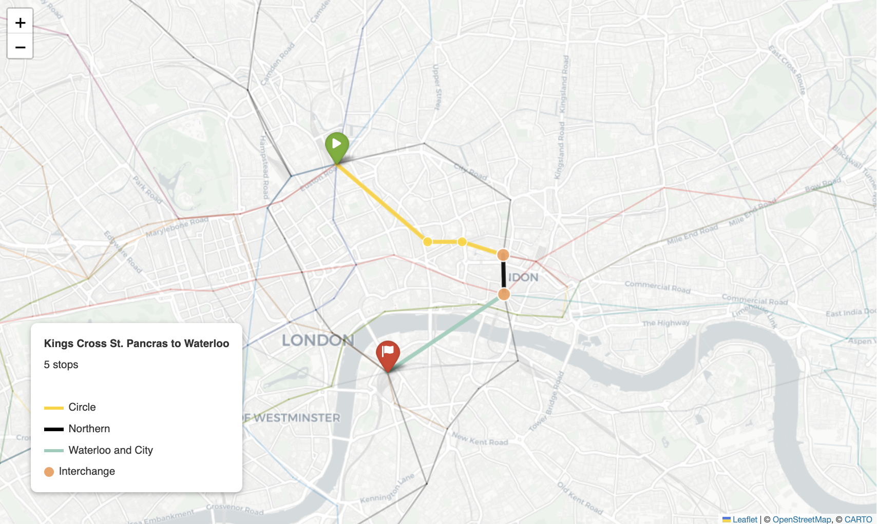
Figure 1-1. Kings Cross to Waterloo.
One naming note: the dataset uses "Kings Cross St. Pancras" without an apostrophe. Passing "King's Cross St. Pancras" returns no result – worth checking if your shortest path queries come back empty. Note also that the route reflects the connections in the dataset rather than the TfL journey planner, which may suggest a different path.
Isochrone – Reachable Stations
An isochrone shows all stations reachable within a given number of stops from a starting point. This is a variable-depth traversal – exactly the kind of query that relational databases handle poorly and Neo4j handles naturally:
CYPHER_ISO = f"""
MATCH p = (origin:Station {{name: $origin}})-[:CONNECTS_TO*1..{ISO_MAX_HOPS}]->(s:Station)
WITH s, min(length(p)) AS hops
RETURN s.name AS name,
       s.lat  AS lat,
       s.lon  AS lon,
       s.zone AS zone,
       hops
ORDER BY hops
"""
Note the directed -> in the pattern – the bidirectional relationships mean this traversal fans out correctly without needing an undirected match. We filter out the origin station from the results after the query:
iso_df = iso_df[iso_df["name"] != ISO_ORIGIN].reset_index(drop=True)
Visualizing the Isochrone
Rather than coloring individual station markers by hop count, we compute convex hull polygons for each hop tier and draw them as filled rings on the map. This gives a much cleaner sense of how the reachable area expands stop by stop:
from scipy.spatial import ConvexHull
import numpy as np

for hop in sorted(iso_df["hops"].unique(), reverse=True):
    tier = iso_df[iso_df["hops"] <= hop]
    coords = np.array([
        (float(lon), float(lat))
        for lon, lat in zip(tier["lon"], tier["lat"])
    ])
    if len(coords) >= 3:
        hull = ConvexHull(coords)
        hull_pts = coords[hull.vertices].tolist()
        hull_pts.append(hull_pts[0])  # close the polygon
        folium.Polygon(
            locations=[[p[1], p[0]] for p in hull_pts],
            color=HOP_COLORS[hop],
            fill=True,
            fill_color=HOP_COLORS[hop],
            fill_opacity=0.12,
            weight=1.5
        ).add_to(m)
We draw hulls from the outermost hop inward so that inner rings are rendered on top of outer ones. Stations not reachable within the maximum hop count are shown as small grey markers for context.
From Oxford Circus at eight hops, the network fans out further west and south than east – the asymmetry of the Underground’s radial structure made visible by the data, as shown in Figure 1-2.
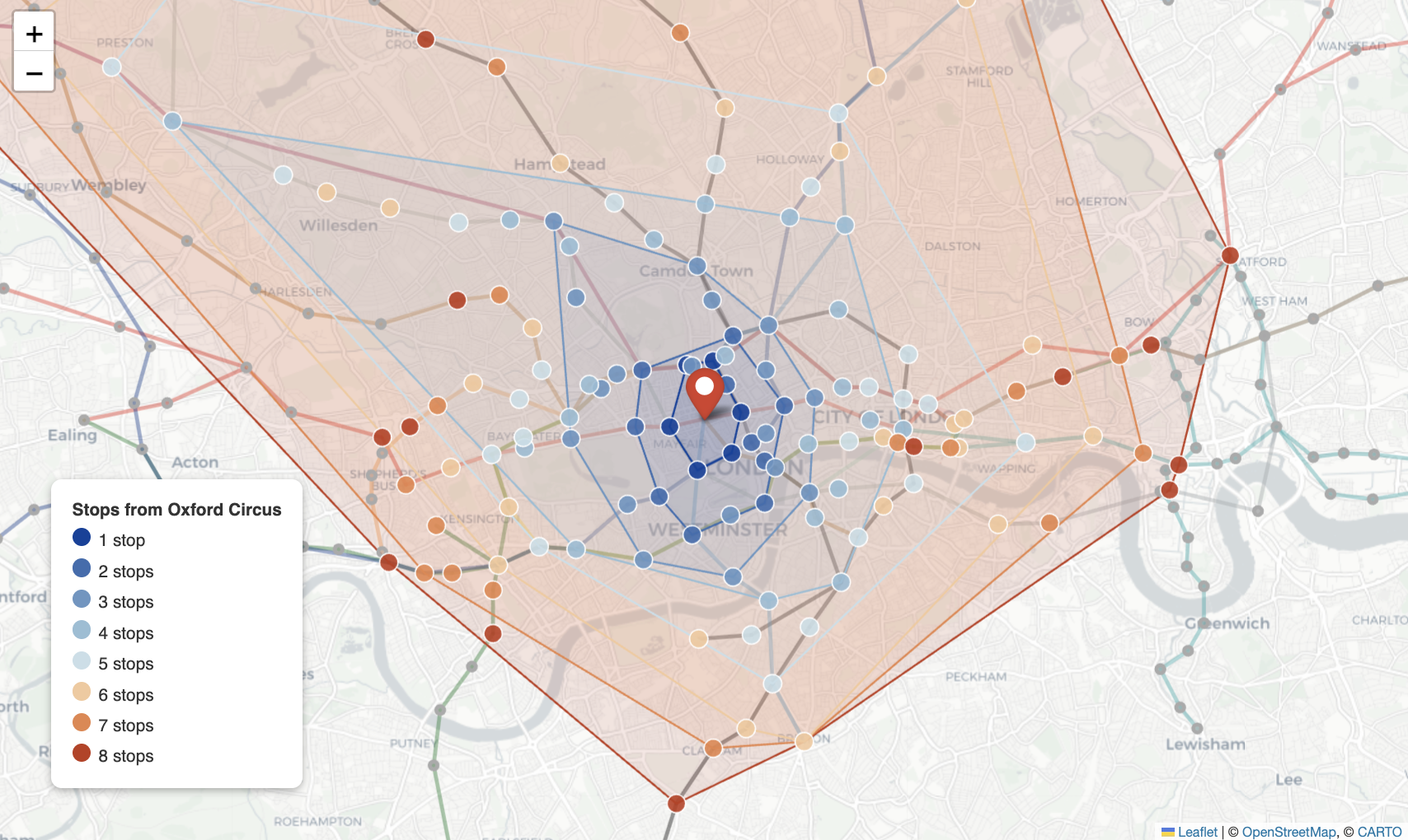
Figure 1-2. Isochrone Map.
Zone Mismatch Analysis
The zone mismatch analysis surfaces the structural tension between TfL’s fare zones – which imply geographic equivalence – and the actual tube network, which is radially organized around central London.
We run the analysis in two passes. First, same-zone pairs: we sample up to 15 stations per zone, generate all pairs within each zone and batch the shortest path queries using UNWIND:
CYPHER_SP_BATCH = """
UNWIND $pairs AS pair
MATCH p = shortestPath(
    (a:Station {name: pair.name_a})-[:CONNECTS_TO*]-(b:Station {name: pair.name_b})
)
RETURN pair.name_a AS station_a,
       pair.name_b AS station_b,
       length(p)   AS hops
"""
We filter to stations with integer zone values only – dropping composite zones like "3,4,5,6" – before sampling:
zone_stations = stations_df[
    stations_df["Zone"].astype(str).str.match(r"^\d+$")
].copy()
zone_stations["ZoneInt"] = zone_stations["Zone"].astype(int)
The same batch query runs for cross-zone pairs: stations in adjacent zones sampled from the same pool. The cross-zone results that have two or fewer hops are the counterintuitive ones – stations that TfL prices differently but which are physically one stop apart.
We visualize same-zone pairs as a box plot of hop counts per zone, which shows that zones further from the centre have wider distributions – more variance in how far apart same-zone stations actually are on the network. Cross-zone anomalies are mapped as teal lines connecting station pairs that are very close on the network but on opposite sides of a zone boundary.
The Streamlit App
The Streamlit application has two tabs. The Shortest Path tab lets users pick any two stations from dropdown menus, displays a summary of stops, lines and interchanges, and renders the route on a Folium map with each segment colored by tube line. The Isochrone tab lets users pick a starting station and a maximum stop count, then renders the convex hull rings on a Folium map alongside a table of reachable station counts by hop.
The zone mismatch analysis is notebook-only – it involves sampling, batching and chart types that work better in a notebook context than in an interactive app.
Folium maps render inside Streamlit via st.iframe:
st.iframe(m._repr_html_(), height=600)
The CartoDB tile URL uses double curly braces around the Folium template variables in an f-string:
MAP_TILES = (
    f"https://{{s}}.basemaps.cartocdn.com/light_all/{{z}}/{{x}}/{{y}}.png?key={CARTO_API_KEY}"
    if CARTO_API_KEY
    else "CartoDB positron"
)
The double braces prevent Python’s f-string parser from treating {s}, {z}, {x} and {y} as format arguments – they’re Folium’s own template placeholders and need to be passed through as literal curly-brace strings.
What You’d Hit in Production
Graph algorithms beyond shortest path. Cypher’s shortestPath() finds the minimum-hop path, which is all this dataset supports. Weighted shortest path – minimizing journey time rather than stop count – requires travel time data on each connection and the Graph Data Science library, available on paid Aura tiers or self-hosted deployments. For the Underground, hop count is a reasonable proxy for journey time given the network’s regularity, but for sparser or more varied networks weighted traversal would give meaningfully different results.
Convex hull edge cases. The scipy.spatial.ConvexHull computation fails if fewer than three points are available for a given hop tier. The notebook wraps it in a try-except, which is the right approach. In production you’d want to log these cases – a single-point or two-point tier is worth knowing about.
Zone composite strings. Several stations have zone values like "3,4,5,6" that require filtering before zone-based analysis. This is a data quality quirk specific to this dataset, but it’s a reminder that real-world graph data rarely arrives perfectly clean. The regex r"^\d+$" cleanly separates single-integer zones from composite ones.
Relationship naming. The relationships in this chapter are CONNECTS_TO. It’s easy to write CONNECTED_TO by habit – they look similar and Neo4j won’t error, it’ll just return no results. If a Cypher query comes back empty when you expect results, check the relationship type first.
Going Further
The native graph model is the foundation for everything that follows in this book. The connections between entities – modeled as relationships – are what make graph traversal fast and Cypher expressive. But a graph database that only stores topology is only part of the picture.
In the chapters ahead we’ll add capabilities to the nodes and relationships themselves: full-text search over document content in chapter 2, geospatial indexing over coordinates in chapter 3, temporal reasoning over time series in chapter 4. Each capability extends what you can express in a Cypher query without leaving Neo4j. By chapter 7, we’ll be combining graph traversal with vector similarity in a single query – and the groundwork for that combination starts here, with understanding what the graph model makes natural and fast.
Chapter 2: Full-Text Search
What Is It?
Neo4j ships with Apache Lucene built in, giving you full-text search – phrase matching, fuzzy matching, relevance scoring – without a separate service. When your data are already in a graph, that search becomes an entry point into something a standalone search engine can’t do: you find your initial results with Lucene, then traverse the graph to discover what surrounds them.
The full-text index in Neo4j is created with a single Cypher procedure call and covers one or more properties across one or more node labels. Queries against it use Lucene’s query syntax – single terms, quoted phrases, boolean operators, fuzzy matching with ~ – and return nodes ranked by BM25 relevance score. The higher the score, the closer the match.
What makes this distinctive is the combination with graph traversal. A standalone search engine returns documents. Neo4j returns nodes – and nodes are connected to other nodes by relationships. A full-text search that finds a paper can immediately extend into a Cypher query that follows citation links, finds co-authors, or surfaces papers that are frequently cited alongside the result. That combination, in a single Cypher statement, is what sets Neo4j’s full-text search apart from running a search engine alongside a database.
When Would You Reach for It?
Full-text search in Neo4j earns its place when the text you’re searching is embedded in a graph and the graph structure is part of what you want to explore. Research literature is the canonical example: papers are text-heavy entities, but the citations between them form a network that carries as much signal as the content itself.
Reach for Neo4j’s full-text search when:
- Your text entities have relationships to other entities that matter for the query
- You want to combine keyword or phrase search with graph traversal in a single operation
- You need relevance-ranked results with BM25 scoring
- You’re already using Neo4j and don’t want to maintain a separate search index
If you’re building a standalone search engine over billions of documents with no graph component, a dedicated search platform is the better choice. But for connected text – papers that cite each other, articles linked by authorship, tickets connected by dependency – Neo4j’s full-text search is a natural fit.
The Use Case
For this chapter we’ll build a research paper discovery tool. Users can search for papers by keyword, phrase or fuzzy match, filter results by field, year or citation count and then traverse the citation graph from any result to discover related work. The traversal options include following outgoing citations, incoming citations, other papers by the same authors and papers that are co-cited alongside the top result.
The Data
We use the same synthetic 200-paper research dataset from the Weaviate chapter of Seven Vector Databases in Seven Days – identical fields, venues, author names, abstract templates and random seed – so the papers are directly comparable across both books. Two things are added that the Weaviate version didn’t have: Author nodes connected to papers via AUTHORED relationships and CITES relationships between papers, with a citation bias toward papers in the same or adjacent research fields.
The graph has two node types:
Paper– withpaper_id,title,abstract,field,venue,yearandcitation_countpropertiesAuthor– with anameproperty
And two relationship types:
(Author)-[:AUTHORED]->(Paper)(Paper)-[:CITES]->(Paper)– with citations biased toward same-field or adjacent-field papers and only toward papers with lower IDs (older papers)
The abstract and title properties are the target for full-text search. The structured fields – field, year, citation_count – serve as filters.
Building the Application
Prerequisites
You’ll need a Neo4j Aura free-tier instance with the connection details stored as environment variables.
Loading the Graph
We clear the database before each run. To avoid transaction timeouts on Aura, we drop constraints and indexes first, then delete nodes in batches of 1,000:
# Drop all constraints
constraints = session.run("SHOW CONSTRAINTS YIELD name RETURN name").data()
for con in constraints:
    session.run(f"DROP CONSTRAINT {con['name']} IF EXISTS")

# Drop all non-system indexes
indexes = session.run(
    "SHOW INDEXES YIELD name, type WHERE type <> 'LOOKUP' RETURN name"
).data()
for idx in indexes:
    session.run(f"DROP INDEX {idx['name']} IF EXISTS")

# Delete in batches
while True:
    result = session.run("""
        MATCH (n) WITH n LIMIT 1000
        DETACH DELETE n
        RETURN count(*) AS deleted
    """)
    if result.single()["deleted"] == 0:
        break
A simple MATCH (n) DETACH DELETE n works for small graphs but can time out on Aura when there are many nodes. The batched approach is safer and worth using as a habit.
We then load in three passes – papers, authors and authorship, citations:
# Paper nodes
session.run("""
    UNWIND $records AS r
    CREATE (p:Paper {
        paper_id:       r.paper_id,
        title:          r.title,
        year:           r.year,
        field:          r.field,
        venue:          r.venue,
        citation_count: r.citation_count,
        abstract:       r.abstract
    })
""", records=paper_records)

# Author nodes and AUTHORED relationships
# MERGE on Author so each author name becomes one node across all papers
session.run("""
    UNWIND $records AS r
    MERGE (a:Author {name: r.author_name})
    WITH a, r
    MATCH (p:Paper {paper_id: r.paper_id})
    CREATE (a)-[:AUTHORED]->(p)
""", records=author_records)

# CITES relationships
session.run("""
    UNWIND $citations AS c
    MATCH (from:Paper {paper_id: c.from_id})
    MATCH (to:Paper   {paper_id: c.to_id})
    CREATE (from)-[:CITES]->(to)
""", citations=citations)
Creating the Full-Text Index
A single procedure call creates a Lucene index over both title and abstract:
session.run("""
    CREATE FULLTEXT INDEX paper_fulltext IF NOT EXISTS
    FOR (p:Paper)
    ON EACH [p.title, p.abstract]
""")
The index is created asynchronously. We poll until it’s ONLINE before querying:
for _ in range(30):
    result = session.run("""
        SHOW INDEXES YIELD name, state
        WHERE name = 'paper_fulltext'
        RETURN state
    """)
    state = result.single()["state"]
    if state == "ONLINE":
        break
    time.sleep(1)
Basic Full-Text Search
Querying the index uses db.index.fulltext.queryNodes. It returns nodes ranked by BM25 score:
def search_papers(query: str, top_k: int = 5):
    with driver.session(database=NEO4J_DATABASE) as session:
        results = session.run("""
            CALL db.index.fulltext.queryNodes('paper_fulltext', $search_query)
            YIELD node AS p, score
            RETURN p.title          AS title,
                   p.field          AS field,
                   p.year           AS year,
                   p.citation_count AS citation_count,
                   score
            ORDER BY score DESC
            LIMIT $top_k
        """, search_query=query, top_k=top_k)
Note the parameter name: search_query, not query. The Neo4j Python driver reserves query as the keyword argument for the Cypher string itself. Using query=... in the keyword arguments conflicts with the driver internals and causes an error. Use search_query, q or any other name.
Keyword, Phrase and Fuzzy Search
Lucene’s full query syntax is available. The three most useful modes for discovery:
Keyword – individual terms scored independently. A query for graph neural networks returns papers containing any of those words, with higher scores for more matches:
search_papers("graph neural networks")
Phrase – wrapping in double quotes requires the words to appear together in that order:
search_papers('"graph neural networks"')
Fuzzy – appending ~ to a term enables edit-distance matching. Useful for misspelled terms or variant spellings:
# 'tranformer' matches 'transformer'
search_papers("tranformer~")
The notebook includes a compare_search_modes() function that runs the same query in both keyword and phrase mode and plots the BM25 scores side by side. This makes the scoring difference concrete: phrase mode scores are generally lower and more selective, while keyword mode casts a wider net with more variance in relevance.
Figure 2-1 shows the score difference for the query graph neural networks.
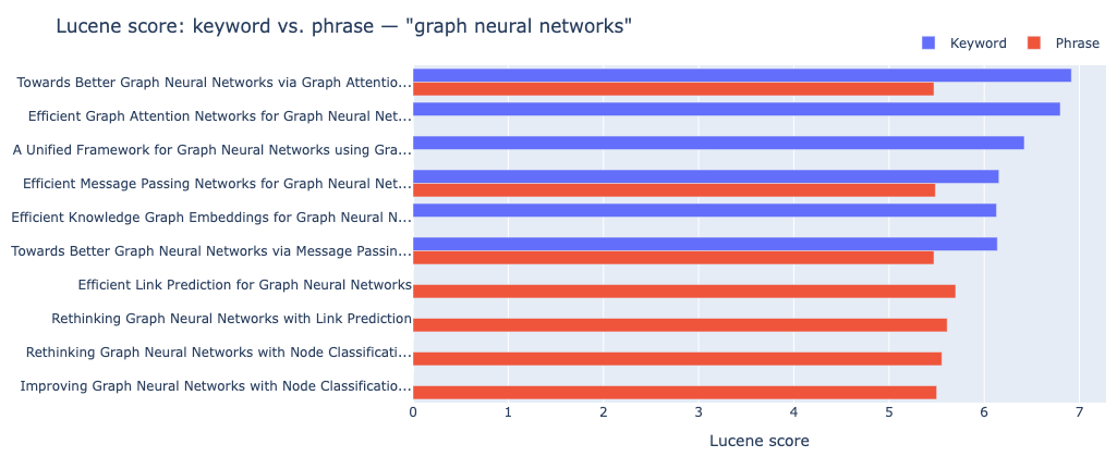
Figure 2-1. Keyword vs. Phrase Search.
Filtered Search
Full-text search narrows by relevance; structured filters narrow by property. The two compose naturally in Cypher with a WHERE clause after the YIELD:
cypher = f"""
    CALL db.index.fulltext.queryNodes('paper_fulltext', $search_query)
    YIELD node AS p, score
    {where_clause}
    RETURN p.title, p.field, p.year, p.citation_count, score
    ORDER BY score DESC
    LIMIT $top_k
"""
Where where_clause is built dynamically from whichever filters are active – field, minimum year, minimum citation count. The Lucene index does the text matching first; the WHERE clause filters the resulting nodes. This is the same pattern as filtered vector search in chapter 6 and chapter 7.
Search Then Traverse: The Graph Layer
This is where Neo4j’s full-text search separates itself from a standalone search engine. Once we have a top-scoring paper, we can immediately traverse the graph from it.
Papers it cites – follow outgoing CITES edges from the top result to see what it builds on:
session.run("""
    CALL db.index.fulltext.queryNodes('paper_fulltext', $search_query)
    YIELD node AS p, score
    WITH p, score ORDER BY score DESC LIMIT 1
    MATCH (p)-[:CITES]->(cited:Paper)
    RETURN p.title AS source_title, cited.title AS cited_title,
           cited.field AS cited_field, cited.citation_count AS cited_citations
    ORDER BY cited.citation_count DESC
    LIMIT $top_k
""", search_query=query, top_k=top_k)
Papers that cite it – traverse incoming CITES edges to find papers that considered this work important enough to build on:
MATCH (citing:Paper)-[:CITES]->(p)
Other work by the same authors – traverse from the paper to its authors, then to their other papers. This path doesn’t exist in a standalone search index at all:
MATCH (a:Author)-[:AUTHORED]->(p)
MATCH (a)-[:AUTHORED]->(other:Paper)
WHERE other <> p
Co-cited papers – find papers that are frequently cited alongside the top result. Two papers are co-cited when a third paper cites both. Papers that are often co-cited tend to address the same problem or be considered foundational in the same area – a relationship that appears nowhere in the papers themselves, only in how others use them:
MATCH (citing:Paper)-[:CITES]->(p)
MATCH (citing)-[:CITES]->(cocited:Paper)
WHERE cocited <> p
WITH p, cocited, count(citing) AS shared_citations
RETURN cocited.title, shared_citations
ORDER BY shared_citations DESC
Citation Network Visualization
The citation network around a top result is visualized as an interactive Plotly graph. The top-scoring paper is the red central node. Blue nodes are papers it cites (outgoing edges). Green nodes are papers that cite it (incoming edges). Node size reflects citation count.
The network is built with NetworkX and rendered with Plotly:
G = nx.DiGraph()
G.add_node(root_id, title=root_title, cc=root_cc, role="root")

for n in edges_raw["out_nodes"]:
    G.add_node(n["id"], title=n["title"], cc=n["cc"], role="cited")
    G.add_edge(root_id, n["id"])

for n in edges_raw["in_nodes"]:
    G.add_node(n["id"], title=n["title"], cc=n["cc"], role="citing")
    G.add_edge(n["id"], root_id)

pos = nx.spring_layout(G, seed=42, k=0.3)
color_map = {"root": "#EF553B", "cited": "#636EFA", "citing": "#00CC96"}
Figure 2-2 shows an example citation network.
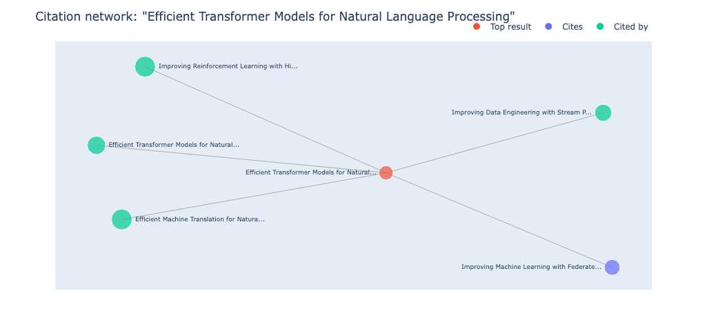
Figure 2-2. Citation Network.
The Streamlit App
The application has two tabs. The Search tab accepts a query string and exposes the three search modes (Keyword, Phrase, Fuzzy) as a radio button, optional filters (field, year, citation count) in a collapsible expander and a results count slider. Results are displayed as cards with title, field, venue, year, citation count and Lucene score, with a horizontal bar chart showing the score distribution across all results.
The Explore tab runs a search and then applies one of four traversal types: Papers it cites, Papers that cite it, Other work by same authors, Co-cited papers. A “Show citation network” button below the traversal results builds and displays the red-blue-green citation network graph.
Both tabs use st.session_state to persist results across re-runs. The Explore tab also clears the cached network figure when a new search is run, so the graph doesn’t show stale results from a previous query.
What You’d Hit in Production
Index freshness. Lucene indexes in Neo4j are updated synchronously on write – new nodes are indexed as soon as they’re created. For bulk ingestion, creating the index after loading is faster than having the index update on every write.
Query syntax errors. A malformed Lucene query – an unmatched quote, a reserved character like + or ! without escaping – throws an exception. The app should sanitize user input or wrap the query call in a try-except before passing it to db.index.fulltext.queryNodes.
Fuzzy matching cost. Fuzzy queries with ~ scan a wider set of index terms and are slower than exact term queries. For interactive search over 200 papers this is imperceptible, but for millions of documents you’d want to set an explicit edit distance (~1 or ~2) rather than relying on the default.
The query parameter. This is worth repeating because it’s easy to hit and the error message isn’t immediately obvious: never use query as a Cypher parameter name when using the Neo4j Python driver. It conflicts with the driver’s own keyword argument for the Cypher string. Use search_query or any other name.
Batched deletion. The simple MATCH (n) DETACH DELETE n pattern can time out on Aura for graphs with tens of thousands of nodes. Batching deletes in groups of 1,000 is more reliable and should be the default approach for database clearing in notebooks that might be re-run.
Going Further
Full-text search surfaces papers by content. Graph traversal extends those results through citation links and authorship. But both of these approaches are vocabulary-dependent – a search for “neural network” won’t naturally surface a paper that uses “deep learning” throughout without ever using the phrase “neural network.”
Chapter 6 addresses this with vector search: by embedding the abstract as a high-dimensional vector, we can find papers that are semantically similar even when they use different vocabulary. And chapter 7 takes the combination further – using vector search to find suspicious transactions and graph traversal to confirm whether they form a ring. The pattern of combining a search capability with graph traversal is one that recurs throughout this book, and it starts here.
Chapter 3: Geospatial
What Is It?
Neo4j supports native geospatial data through its point type – a first-class property that stores 2D or 3D coordinates and enables spatial queries directly in Cypher. Rather than computing distances in application code, you can ask the database: which cities are within 150 km of Barcelona? Which cross-border pairs are geographically closest? The answer comes back as a graph traversal, not a table scan.
The point type integrates with Neo4j’s indexing infrastructure. A point index on a property enables efficient spatial range queries and proximity lookups. You create it the same way as any other index and Cypher’s spatial functions work against it automatically.
What makes this distinctive is the combination with graph structure. Geographic proximity is one kind of relationship between places. But places also have relationships to each other through the network – neighboring cities, shared air corridors, administrative boundaries. Neo4j lets you query both at once: find all cities within a radius using point.distance(), then traverse the pre-computed NEIGHBORS graph to explore cross-border connectivity. Both in a single Cypher statement.
When Would You Reach for It?
Geospatial queries in Neo4j earn their place when location is one dimension of a richer graph. Pure geospatial problems – mapping, routing, satellite imagery – belong in dedicated GIS platforms. But when your entities have both a location and a network of relationships and you need to query across both, Neo4j handles this naturally.
Reach for Neo4j’s geospatial capability when:
- Your entities have coordinates and also have meaningful relationships to each other
- You want to combine proximity queries with graph traversal in a single operation
- You’re already using Neo4j and adding spatial queries doesn’t justify a second system
- You’re asking questions like “find the nearest X, then follow the graph from there”
Environmental monitoring is a strong use case: monitoring stations have locations, but air quality also spreads through corridors, follows wind patterns and crosses administrative borders. Both the spatial and the network dimension matter.
The Use Case
For this chapter we’ll explore air quality data along the Pyrenees corridor – the mountain range that forms the border between France and Spain. We fetch real air quality and weather readings from the IQAir API for cities in two French regions (Occitanie and Nouvelle-Aquitaine) and three Spanish regions (Aragon, Catalonia and Navarre), load them into Neo4j with coordinates stored as native point types and then query across both dimensions: which cities are nearest to a reference city, which French-Spanish pairs are geographically close, which neighboring pairs have the biggest pollution difference and which city is most central to the corridor network.
The Data
Air quality readings come from the IQAir API. A free API key is sufficient – the free tier allows five requests per minute and the ingest notebook spaces calls 12 seconds apart to stay within that limit.
Each city produces a Reading node with: aqi_us (the US AQI value), aqi_category (Good through Hazardous), main_pollutant, temperature, humidity, wind_speed and timestamp.
The graph model is:
(:City {name, country, state, location})
  -[:HAS_READING]->
(:Reading {timestamp, aqi_us, aqi_category, main_pollutant,
           temperature, humidity, wind_speed})
NEIGHBORS relationships connect cities within 200 km of each other, computed once at ingest time using point.distance() in Cypher.
Figure 3-1 shows the corridor at a glance – green markers indicate Good air quality, yellow Moderate, with marker size reflecting AQI value.
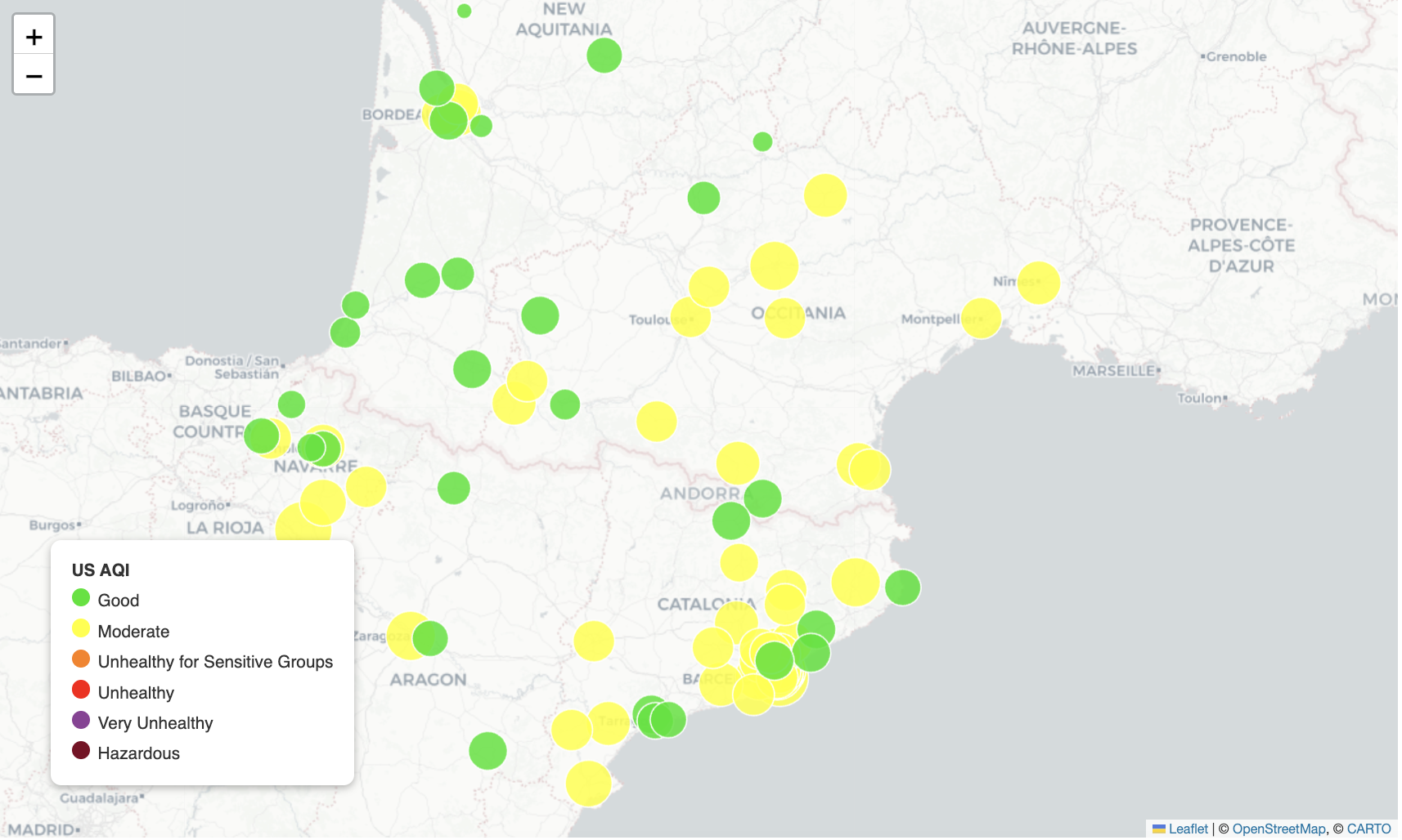
Figure 3-1. Air Quality across the Pyrenees Corridor.
Building the Application
Prerequisites
You’ll need a Neo4j Aura free-tier instance with the connection details stored as environment variables.
The chapter also uses CartoDB basemap tiles for the Folium maps. CartoDB now requires a free API key, available at carto.com/basemaps/apikey, stored as CARTO_API_KEY. The Streamlit app degrades gracefully if the key is absent, falling back to the default CartoDB Positron tile set.
Loading the data. The repo includes a pre-populated Aura backup file (03_aqi_geospatial.backup). The fastest way to get started is to import it into your Aura instance directly: open the Aura console, select your instance, go to … > Restore from File and upload the backup file. Once the import completes, the database is ready and you can skip straight to 03_aqi_geospatial.ipynb.
If you’d prefer to fetch fresh data yourself – or want to extend the city list – run 03_aqi_ingest.ipynb instead. You’ll need an additional IQAir API key stored as IQAIR_API_KEY and the ingest takes ~20 minutes due to the IQAir free-tier rate limit of five requests per minute.
Storing Coordinates as Points
The uniqueness constraint on City uses a composite key – name and country together – because the same city name can appear in both France and Spain:
session.run("""
    CREATE CONSTRAINT city_unique IF NOT EXISTS
    FOR (c:City) REQUIRE (c.name, c.country) IS UNIQUE
""")

session.run("""
    CREATE POINT INDEX city_location IF NOT EXISTS
    FOR (c:City) ON (c.location)
""")
Cities are loaded with MERGE so the notebook is safe to re-run as new readings accumulate. Coordinates are stored as a native Neo4j point:
session.run("""
    MERGE (c:City {name: $city, country: $country})
    SET c.state    = $state,
        c.location = point({latitude: $lat, longitude: $lon})
""", **record)
Each API call produces a new Reading node timestamped at the time of the fetch. Readings accumulate over time – running the ingest notebook daily builds a time series of air quality readings per city.
Computing NEIGHBORS in Cypher
The NEIGHBORS relationship is computed entirely in Cypher using point.distance(). No Python distance calculation needed:
session.run("""
    MATCH (a:City), (b:City)
    WHERE elementId(a) < elementId(b)
      AND point.distance(a.location, b.location) / 1000 <= $max_km
    WITH a, b,
         round(point.distance(a.location, b.location) / 1000, 1) AS distance_km
    MERGE (a)-[r:NEIGHBORS]-(b)
    SET r.distance_km = distance_km
    RETURN count(*) AS neighbors_created
""", max_km=NEIGHBOR_DISTANCE_KM)
elementId(a) < elementId(b) deduplicates pairs – without it, every city pair generates two relationships. MERGE rather than CREATE means running the ingest notebook again won’t create duplicate relationships.
Extracting Coordinates from Point Properties
When reading point properties back in Cypher, we access latitude and longitude with dot notation on the point value:
result = session.run("""
    MATCH (c:City)-[:HAS_READING]->(r:Reading)
    WITH c, r ORDER BY r.timestamp DESC
    WITH c, collect(r)[0] AS latest
    RETURN c.name                AS city,
           c.country             AS country,
           c.location.latitude   AS lat,
           c.location.longitude  AS lon,
           latest.aqi_us         AS aqi_us,
           latest.aqi_category   AS aqi_category,
           latest.main_pollutant AS main_pollutant,
           latest.temperature    AS temperature,
           latest.humidity       AS humidity,
           latest.wind_speed     AS wind_speed
""")
The collect(r)[0] pattern retrieves the most recent reading per city by sorting by timestamp descending first, then taking the first element of the collected list. This is a common Neo4j idiom for “latest record per group.”
Query 1: Cities Within Radius
The proximity query uses point.distance() in the WHERE clause. The function returns meters, so we divide by 1000 for kilometers:
result = session.run("""
    MATCH (ref:City {name: $city, country: $country})
    MATCH (c:City)-[:HAS_READING]->(r:Reading)
    WITH ref, c, r ORDER BY r.timestamp DESC
    WITH ref, c, collect(r)[0] AS latest
    WHERE c <> ref
      AND point.distance(ref.location, c.location) / 1000 <= $radius_km
    RETURN c.name AS city,
           c.country AS country,
           round(point.distance(ref.location, c.location) / 1000, 1) AS distance_km,
           latest.aqi_us AS aqi_us,
           latest.aqi_category AS aqi_category
    ORDER BY distance_km
""", city=city, country=country, radius_km=radius_km)
Query 2: Cross-Border Neighbors
This query traverses the pre-computed NEIGHBORS graph to find French-Spanish city pairs, then joins the latest reading for each:
result = session.run("""
    MATCH (a:City)-[n:NEIGHBORS]-(b:City)
    WHERE a.country = 'France' AND b.country = 'Spain'
    MATCH (a)-[:HAS_READING]->(ra:Reading)
    MATCH (b)-[:HAS_READING]->(rb:Reading)
    WITH a, b, n, ra, rb ORDER BY ra.timestamp DESC, rb.timestamp DESC
    WITH a, b, n, collect(ra)[0] AS latest_a, collect(rb)[0] AS latest_b
    RETURN a.name AS french_city,
           b.name AS spanish_city,
           n.distance_km AS distance_km,
           latest_a.aqi_us AS aqi_france,
           latest_b.aqi_us AS aqi_spain,
           abs(latest_a.aqi_us - latest_b.aqi_us) AS aqi_diff
    ORDER BY distance_km
""")
This is spatial and graph combined in one query: the NEIGHBORS relationship was built using spatial distance at ingest time, and we traverse it here like any other graph relationship.
Figure 3-2 maps the result. Each line connects a French city to a Spanish city within 100 km, making the corridor structure immediately visible – the border in the west and the cluster in the east are the most densely connected sections.
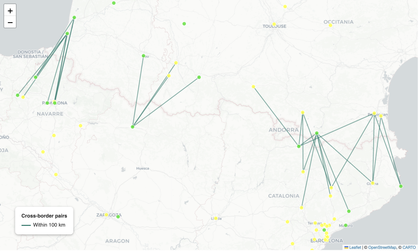
Figure 3-2. Cross-Border City Pairs.
Query 3: AQI Gradient Pairs
Which neighboring city pairs have the biggest difference in air quality? Pollution doesn’t respect geography – cities close together can have very different AQI readings:
result = session.run("""
    MATCH (a:City)-[n:NEIGHBORS]-(b:City)
    WHERE elementId(a) < elementId(b)
    MATCH (a)-[:HAS_READING]->(ra:Reading)
    MATCH (b)-[:HAS_READING]->(rb:Reading)
    WITH a, b, n, ra, rb ORDER BY ra.timestamp DESC, rb.timestamp DESC
    WITH a, b, n, collect(ra)[0] AS latest_a, collect(rb)[0] AS latest_b
    WITH a.name AS city_a, a.country AS country_a,
         b.name AS city_b, b.country AS country_b,
         n.distance_km AS distance_km,
         latest_a.aqi_us AS aqi_a, latest_b.aqi_us AS aqi_b,
         abs(latest_a.aqi_us - latest_b.aqi_us) AS aqi_diff
    RETURN city_a, country_a, city_b, country_b,
           distance_km, aqi_a, aqi_b, aqi_diff
    ORDER BY aqi_diff DESC
    LIMIT 10
""")
Query 4: Most Connected City
Which city has the most neighbors within the corridor? This is the most geographically central city in the network:
result = session.run("""
    MATCH (c:City)-[:NEIGHBORS]-(neighbor:City)
    RETURN c.name AS city, c.country AS country,
           count(*) AS neighbor_count
    ORDER BY neighbor_count DESC
    LIMIT 10
""")
Mapping the Data
The AQI map uses the standard US AQI color scale:
AQI_COLORS = {
    "Good":                           "#00E400",
    "Moderate":                       "#FFFF00",
    "Unhealthy for Sensitive Groups": "#FF7E00",
    "Unhealthy":                      "#FF0000",
    "Very Unhealthy":                 "#8F3F97",
    "Hazardous":                      "#7E0023",
}
City markers are sized proportionally to AQI value – larger circles indicate worse air quality – and colored by category. The NEIGHBORS overlay adds lines between cities, with cross-border pairs within 100 km highlighted distinctly.
The geospatial notebook also includes an AQI distribution box plot by country, a top-10 cities bar chart colored by AQI category and an AQI vs temperature scatter plot to explore whether temperature correlates with air quality across the corridor.
The Streamlit App
The app is a single-screen layout with a sidebar. The sidebar lets users pick a reference city from a dropdown (defaulting to Barcelona, Spain), set a radius in kilometers and a minimum AQI filter. Clicking “Find nearby cities” runs the spatial query and displays summary metrics (reference AQI, nearby city count, average AQI nearby, highest AQI nearby), a Folium map with a dashed radius circle, lines to each nearby city colored by AQI category and a horizontal bar chart of nearby cities sorted by AQI.
The map renders via st.iframe:
st.iframe(m._repr_html_(), height=520)
A collapsible data table shows the full results including distance, AQI, category, main pollutant, temperature, humidity and wind speed for each nearby city.
What You’d Hit in Production
API rate limits. The IQAir free tier allows five requests per minute. The ingest notebook spaces calls 12 seconds apart. If you increase the city list significantly, the ingest run will take proportionally longer. A paid API tier removes the rate limit and allows fetching data for more regions.
Reading accumulation. The ingest notebook is designed to be run repeatedly – each run adds a new Reading node per city. Over time this builds a time series. The “latest reading” pattern (ORDER BY r.timestamp DESC ... collect(r)[0]) retrieves only the most recent reading and is efficient, but the total Reading node count will grow with each ingest run. Consider adding a retention policy if you run the ingest daily over a long period.
The database clear cell. The ingest notebook contains a commented-out cell that clears the database. Run it only on the first run – subsequent runs should accumulate readings, not start from scratch. The cell is clearly marked and commented out by default.
Point property access syntax. The notation c.location.latitude and c.location.longitude accesses the latitude and longitude components of a point property in Cypher. This is easy to get wrong – c.lat would refer to a separate top-level property named lat, which doesn’t exist in this model.
elementId() not id(). Neo4j 5.x deprecated the id() function in favor of elementId(), which returns a string. The NEIGHBORS computation uses elementId(a) < elementId(b) for deduplication. If you see deprecation warnings in other queries, check whether they use id() and update them.
Going Further
Geospatial queries answer “what is near what?” Graph traversal answers “what is connected to what?” In this chapter we used both together – point.distance() to build the neighbor network at ingest time, then graph traversal to explore it at query time. But proximity and connectivity are still properties of the current snapshot.
Chapter 4 adds time. Air quality changes day to day and the same city that reads Good today may read Unhealthy after a weather event. Temporal queries let you ask how a graph has changed over time and what patterns emerge when you look at the data as a sequence of snapshots rather than a single state. That’s where we go next.
Chapter 4: Temporal
What Is It?
Relational databases handle time series as regular rows – a price is just another record in a table, distinguished from other records by a date column. Neo4j handles time series as graph structure: each price is a node, connected to a stock node via a HAS_PRICE relationship. Temporal queries become traversal questions. Start at a stock node, follow its price nodes, filter by date, aggregate. The graph model makes the time dimension as queryable as any other structure in the graph.
Neo4j’s native date and datetime types are first-class values in Cypher. A date property on a node is not stored as a string – it has a structured representation that Cypher understands natively. You filter with WHERE p.date >= date($start), sort chronologically and compute durations with duration.between(). A range index on Price.date makes date-range queries fast regardless of how many price nodes are in the graph.
When Would You Reach for It?
Temporal queries in Neo4j earn their place when time is one dimension of a richer graph rather than the only dimension. Pure time series problems – high-frequency trading data, IoT sensor streams at millisecond resolution – belong in purpose-built time series databases. But when your time-varying data are connected to other entities that carry meaning, Neo4j handles the combination naturally.
Reach for Neo4j’s temporal capability when:
- Your time-varying data are connected to other nodes – issuers, counterparties, events
- You want to combine date-range queries with graph traversal in a single operation
- You need date arithmetic – durations, period comparisons – as part of a graph query
- You’re already using Neo4j and don’t want to add a separate time series store
Financial data are a natural fit: prices are time series, but stocks are connected to each other through shared market behavior and the relationship between two stocks’ price histories is itself a meaningful query.
The Use Case
For this chapter we’ll build a stock price analysis tool for a curated subset of S&P 500 companies. Users can view the full price history for any symbol, display it as a candlestick chart with configurable bucket sizes, overlay 20-day and 50-day moving averages, compare the performance of all symbols across the full five-year period and explore the price correlation between any two symbols.
The Data
We use the S&P 500 historical price dataset from Kaggle, published under CC0 license. The full dataset covers 505 symbols from February 2013 to February 2018. We load a curated subset of 150 symbols across major sectors – Technology, Financials, Healthcare, Consumer and others – which keeps the total node count comfortably within Aura’s free-tier limit of 200,000 nodes.
The graph model is:
(:Stock {symbol})-[:HAS_PRICE]->(:Price {date, open, high, low, close, volume})
Stock nodes carry only the symbol property. Price nodes carry the full OHLCV data for one trading day. At 150 symbols over roughly 1,260 trading days each, the graph contains around 189,000 Price nodes.
Building the Application
Prerequisites
You’ll need a Neo4j Aura free-tier instance with the connection details stored as environment variables.
Loading the Graph
We create a uniqueness constraint on Stock.symbol and a range index on Price.date, then load in two passes:
session.run("""
    CREATE CONSTRAINT stock_symbol IF NOT EXISTS
    FOR (s:Stock) REQUIRE s.symbol IS UNIQUE
""")

session.run("""
    CREATE INDEX price_date IF NOT EXISTS
    FOR (p:Price) ON (p.date)
""")

# One Stock node per symbol
session.run("""
    UNWIND $symbols AS sym
    MERGE (:Stock {symbol: sym})
""", symbols=symbols)
Price nodes are loaded in batches of 1,000 rows using UNWIND to keep transaction size manageable:
for chunk in tqdm(chunks(records, CHUNK_SIZE)):
    session.run("""
        UNWIND $rows AS row
        MATCH (s:Stock {symbol: row.symbol})
        CREATE (p:Price {
            date:   date(row.date),
            open:   row.open,
            high:   row.high,
            low:    row.low,
            close:  row.close,
            volume: row.volume
        })
        CREATE (s)-[:HAS_PRICE]->(p)
    """, rows=chunk)
We use CREATE rather than MERGE for price nodes – each date is unique per stock and we’re loading clean data, so MERGE would add overhead without benefit.
Query 1: Price History
The price history query filters by date using Neo4j’s native date() function:
result = session.run("""
    MATCH (s:Stock {symbol: $symbol})-[:HAS_PRICE]->(p:Price)
    WHERE p.date >= date($start) AND p.date <= date($end)
    RETURN p.date  AS date,
           p.open  AS open,
           p.high  AS high,
           p.low   AS low,
           p.close AS close
    ORDER BY p.date
""", symbol=SYMBOL, start=START_DATE, end=END_DATE)
Neo4j returns date values as native Python datetime.date objects. To use them as a pandas datetime index for resampling, convert with pd.to_datetime(df["date"].astype(str)).
Query 2: Candlestick Chart
The daily OHLC data comes back from Neo4j as individual rows. We bucket it into N-day windows in pandas using resample() and agg():
BUCKET_DAYS = 5

ohlc_df = (
    price_df
    .set_index("date")
    .resample(f"{BUCKET_DAYS}D")
    .agg(
        open=("open",  "first"),
        high=("high",  "max"),
        low=("low",   "min"),
        close=("close","last")
    )
    .dropna()
    .reset_index()
)
Each bucket takes the opening price of the first day, the closing price of the last day and the high and low across the entire window. The .dropna() step removes any empty buckets caused by weekends or holidays at period boundaries.
Plotting with Plotly’s go.Candlestick requires one formatting choice: set type="category" on the x-axis. Without it, Plotly treats the date axis as continuous and renders gaps for weekends and holidays as empty space, which makes the chart look sparse. With type="category", each bucket is an equal-width column regardless of the calendar gap:
fig.update_xaxes(
    type="category",
    tickangle=-45,
    tickvals=ohlc_df["date"][::max(1, len(ohlc_df)//12)].astype(str).tolist()
)
Figure 4-1 shows an example using the AAPL symbol.
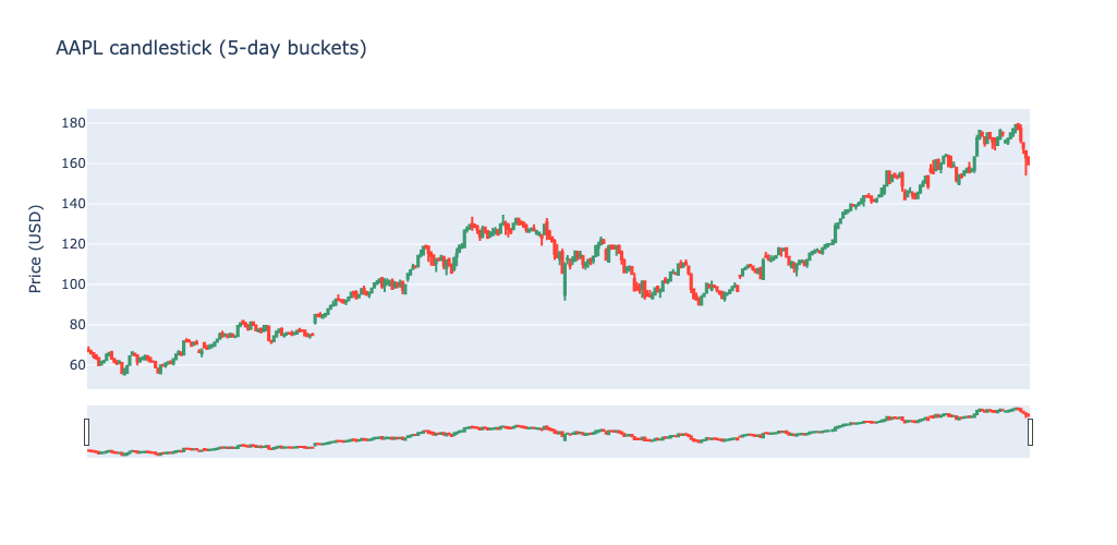
Figure 4-1. AAPL Candlestick.
Query 3: Moving Averages
Moving averages are computed in pandas after retrieving the price series from Neo4j. Cypher has no built-in rolling window function and pandas.Series.rolling() is both cleaner and faster for this purpose:
price_df["ma_20"] = price_df["close"].rolling(window=20).mean()
price_df["ma_50"] = price_df["close"].rolling(window=50).mean()
The 20-day MA captures short-to-medium term trend; the 50-day MA shows the longer-term direction. We overlay both on the closing price as a three-line chart in Plotly.
Figure 4-2 shows an example using the AAPL symbol.
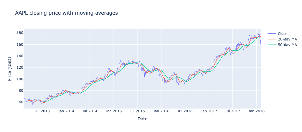
Figure 4-2. AAPL Moving Averages.
Query 4: Best and Worst Performers
The performance query runs entirely in Cypher, using min() and max() on the date to anchor the first and last price nodes:
result = session.run("""
    MATCH (s:Stock)-[:HAS_PRICE]->(p:Price)
    WITH s.symbol AS symbol,
         min(p.date) AS first_date,
         max(p.date) AS last_date
    MATCH (s:Stock {symbol: symbol})-[:HAS_PRICE]->(first:Price {date: first_date})
    MATCH (s)-[:HAS_PRICE]->(last:Price  {date: last_date})
    WITH symbol,
         first.close AS first_price,
         last.close  AS last_price,
         round((last.close - first.close) / first.close * 100, 2) AS pct_change
    RETURN symbol, first_price, last_price, pct_change
    ORDER BY pct_change DESC
""")
The query anchors on min(p.date) and max(p.date) rather than literal start and end dates because different symbols may have different first and last trading days in the dataset – this approach correctly handles any gaps in coverage. The results are displayed as a bar chart of the top 10 and bottom 10 performers, colored green for positive and red for negative returns.
Query 5: Price Correlation
Do two stocks move together? We fetch the closing prices for both symbols on matching dates in a single Cypher query and compute the Pearson correlation in pandas:
result = session.run("""
    MATCH (a:Stock {symbol: $sym_a})-[:HAS_PRICE]->(pa:Price)
    MATCH (b:Stock {symbol: $sym_b})-[:HAS_PRICE]->(pb:Price)
    WHERE pa.date = pb.date
    RETURN pa.date  AS date,
           pa.close AS price_a,
           pb.close AS price_b
    ORDER BY pa.date
""", sym_a=SYMBOL_A, sym_b=SYMBOL_B)

correlation = corr_df["price_a"].corr(corr_df["price_b"])
The WHERE pa.date = pb.date join happens in the graph query itself – Neo4j matches price nodes from both stocks on the same date. We visualize the result as a dual-axis line chart, with each stock on its own y-axis so their price scales don’t interfere.
The Streamlit App
The application has three tabs. The Candlestick tab lets users pick a symbol from a dropdown, a date range, and a bucket size from a sidebar slider. It displays a summary of trading day count, first close and last close, then the candlestick chart. The Moving Average tab shows the same price series with 20-day and 50-day moving averages overlaid. The Performance tab shows the top 10 and bottom 10 performers across the full five-year period as a bar chart, with data tables for each group below.
The sidebar controls – symbol, date range, bucket size – apply to the Candlestick and Moving Average tabs. The Performance tab runs a separate cached query over all symbols and ignores the date range selection.
What You’d Hit in Production
Node count. Aura’s free tier caps at 200,000 nodes. 150 symbols at ~1,260 trading days each produces around 189,000 price nodes, which fits. The full 505-symbol dataset would produce around 636,000 price nodes and requires a paid tier. If you need more symbols, consider whether you need all five years of data or could work with a shorter window.
Candlestick x-axis. The type="category" setting on the x-axis is essential for candlestick charts with date gaps. Without it, Plotly renders weekends and holidays as empty columns, making the chart hard to read. This applies to any OHLC chart with non-continuous dates.
Date conversion. Neo4j returns date values as Python datetime.date objects. Pandas needs them as datetime64 for resample() to work. The conversion pd.to_datetime(df["date"].astype(str)) is reliable and handles any edge cases in the date representation.
Intra-day data. The one-price-per-trading-day model doesn’t extend to intra-day or tick data. Minute-level data for 150 stocks over five years would be around 115 million price nodes – well beyond what Neo4j Aura’s free tier can hold.
Moving averages in Cypher. Computing a rolling mean in pure Cypher is possible but verbose and slow compared to pandas. The division of labor in this chapter – Neo4j for retrieval and filtering, pandas for numerical computation – is the right default for this kind of analytical workload.
Going Further
Prices and dates are structured, numeric data. Every property in chapters 1 through 4 has been a scalar: a name, a coordinate, a date, a number. Chapter 5 explores what happens when nodes need to carry richer, more complex payloads – variable-structure metadata that differs across instances of the same node type. That requires a different approach to property storage and it’s where we go next.
Chapter 5: Document-Style Properties
What Is It?
Neo4j node properties support primitive types – strings, integers, floats, booleans, dates – and arrays of primitives. Nested maps are not supported as native property values. To store heterogeneous, document-style metadata alongside graph structure, the standard approach is to serialize it as a JSON string and parse it back at query time using APOC’s apoc.convert.fromJsonMap() function.
This is a deliberate constraint rather than an oversight. Neo4j’s query engine is optimized for traversal and deeply nested document structures are better handled at the edge between the database and the application rather than inside the graph query itself. The sweet spot is: store rich, variable-structure metadata as a JSON string on the node; use APOC to deserialize it inside Cypher when you need to query or mutate it; promote frequently filtered fields to top-level properties with their own indexes.
APOC (Awesome Procedures On Cypher) is Neo4j’s standard extension library, available on all Aura tiers. It provides apoc.convert.fromJsonMap() to parse a JSON string into a Cypher map, apoc.convert.toJson() to serialize a map back to a string and apoc.map.removeKey() to delete a field from a map without touching the rest.
When Would You Reach for It?
Document-style properties earn their place when your nodes need to carry structured metadata that varies across instances and that metadata doesn’t need to be independently indexed or traversed as graph structure. The key question is whether you need to query inside the property or just store and retrieve it as a unit.
Reach for this pattern when:
- Your nodes carry variable-structure metadata that differs across instances of the same label
- The metadata belongs logically to the node rather than deserving its own node type
- You need to store and retrieve the metadata as a unit, or query inside it occasionally with APOC
- You want to avoid the overhead of a normalized schema for genuinely heterogeneous data
Libraries, product catalogs and content management systems are all cases where some nodes carry rich, variable metadata alongside graph-structured relationships to other entities.
The Use Case
For this chapter we’ll build a small library inventory system with three item types – books, journals and multimedia – each carrying a different metadata structure in the same metadata property on Item nodes. We demonstrate how to query across the three types using APOC, how to traverse the graph to join items with their authors and publishers and how to add and remove fields from stored metadata without rewriting the whole object.
The Data
The inventory is small by design – 15 items, 3 authors and 3 publishers. The point is to show the metadata pattern clearly, not to load data at scale.
The three metadata structures are:
- Books – a flat map:
isbn,pages,language,author_id - Journals – a map with a list:
volume,year,editor,articles[] - Multimedia – a nested map:
format,duration_min,language,contributors{}
All three are stored in the same metadata property on Item nodes.
The graph model is:
(:Publisher {id, name, location})-[:PUBLISHED]->(:Item {id, title, item_type, metadata})
(:Author    {id, name, nationality})-[:AUTHORED]->(:Item)
Building the Application
Prerequisites
You’ll need a Neo4j Aura free-tier instance with the connection details stored as environment variables.
Storing Metadata
The metadata property is stored as a JSON string. In Python, we serialize with json.dumps() before passing to Neo4j:
ITEMS = [
    {"id": 1, "title": "The Quantum Garden", "item_type": "book",
     "publisher_id": 1,
     "metadata": {"isbn": "978-0-123456-47-2", "pages": 320,
                  "language": "English", "author_id": 1}},
    {"id": 6, "title": "Nature Reviews",     "item_type": "journal",
     "publisher_id": 2,
     "metadata": {"volume": 12, "year": 2023, "editor": "Dr. Smith",
                  "articles": ["AI in Medicine", "CRISPR 2024", "Climate Models"]}},
    {"id": 11, "title": "Deep Learning DVD", "item_type": "multimedia",
     "publisher_id": 3,
     "metadata": {"format": "DVD", "duration_min": 145, "language": "English",
                  "contributors": {"director": "Ana Lima", "narrator": "Tom Chen"}}},
]

session.run("""
    UNWIND $rows AS row
    MERGE (i:Item {id: row.id})
    SET i.title     = row.title,
        i.item_type = row.item_type,
        i.metadata  = row.metadata_json
""", rows=[{**item, "metadata_json": json.dumps(item["metadata"])} for item in ITEMS])
We pass the metadata as a JSON string so it’s stored as a single string property. All three item types use the same metadata property name – the structure varies but the storage pattern is uniform.
APOC: Parsing Metadata in Cypher
apoc.convert.fromJsonMap() parses the JSON string back into a Cypher map at query time. Once parsed, you access fields with dot notation and use standard Cypher operators on them:
result = session.run("""
    MATCH (i:Item)
    WHERE i.item_type = 'book'
    WITH i, apoc.convert.fromJsonMap(i.metadata) AS meta
    RETURN i.id          AS id,
           i.title       AS title,
           meta.isbn     AS isbn,
           meta.pages    AS pages,
           meta.language AS language
    ORDER BY i.id
""")
The WITH i, apoc.convert.fromJsonMap(i.metadata) AS meta line is the key pattern. It deserializes the JSON string into a map named meta, which then behaves like any Cypher map for the rest of the query.
Query 1: Books – Flat Metadata
Books have flat metadata – every field is a scalar. meta.isbn, meta.pages and meta.language work as direct property accessors once the JSON is parsed.
Query 2: Journals – Metadata with a List
Journals have an articles list inside the metadata. Cypher’s size() function counts the elements:
result = session.run("""
    MATCH (i:Item)
    WHERE i.item_type = 'journal'
    WITH i, apoc.convert.fromJsonMap(i.metadata) AS meta
    RETURN i.id                AS id,
           i.title             AS title,
           meta.editor         AS editor,
           meta.volume         AS volume,
           meta.year           AS year,
           size(meta.articles) AS article_count
    ORDER BY article_count DESC
""")
Query 3: Multimedia – Nested Map
Multimedia items have a contributors map nested inside the metadata. Returning meta.contributors gives you the whole nested map as a Cypher map value, which the Python driver returns as a Python dict:
result = session.run("""
    MATCH (i:Item)
    WHERE i.item_type = 'multimedia'
    WITH i, apoc.convert.fromJsonMap(i.metadata) AS meta
    RETURN i.id              AS id,
           i.title           AS title,
           meta.format       AS format,
           meta.duration_min AS duration_min,
           meta.language     AS language,
           meta.contributors AS contributors
    ORDER BY i.id
""")
Query 4: Books with Authors – Graph Traversal
Graph traversal and metadata access compose naturally. We follow the AUTHORED relationship to join books with their authors, then access the book metadata in the same query:
result = session.run("""
    MATCH (a:Author)-[:AUTHORED]->(i:Item)
    WITH a, i, apoc.convert.fromJsonMap(i.metadata) AS meta
    RETURN i.id          AS id,
           i.title       AS title,
           a.name        AS author,
           a.nationality AS nationality,
           meta.pages    AS pages,
           meta.language AS language
    ORDER BY a.name, i.id
""")
This is the value proposition of the pattern: graph structure for relationships, JSON strings for variable metadata, APOC to bridge the two.
Query 5: Search Journals by Article Keyword
Cypher’s ANY() function iterates over a list and returns true if any element satisfies a predicate. We use it to search for journals containing a keyword in any article title:
result = session.run("""
    MATCH (i:Item)
    WHERE i.item_type = 'journal'
    WITH i, apoc.convert.fromJsonMap(i.metadata) AS meta
    WHERE ANY(article IN meta.articles WHERE article CONTAINS $keyword)
    RETURN i.id        AS id,
           i.title     AS title,
           meta.editor AS editor,
           [article IN meta.articles WHERE article CONTAINS $keyword]
               AS matching_articles
    ORDER BY i.id
""", keyword=KEYWORD)
The list comprehension [article IN meta.articles WHERE article CONTAINS $keyword] returns only the matching article titles, not the full list. Both ANY() and list comprehensions work on deserialized APOC maps just as they work on native Cypher lists.
Query 6: Adding a Field to Metadata
To add a key to the stored metadata, parse the JSON string, extend the map using Cypher’s map spread operator, then serialize back:
session.run("""
    MATCH (i:Item {id: 1})
    WITH i, apoc.convert.fromJsonMap(i.metadata) AS meta
    SET i.metadata = apoc.convert.toJson(meta {.*, edition: 'Second'})
""")
The meta {.*, edition: 'Second'} syntax creates a new map containing all existing keys (.*) plus the new edition key. apoc.convert.toJson() serializes it back to a string. The original metadata property is replaced with the updated JSON string.
Query 7: Removing a Field from Metadata
To remove a key, use apoc.map.removeKey():
session.run("""
    MATCH (i:Item {id: 1})
    WITH i, apoc.convert.fromJsonMap(i.metadata) AS meta
    SET i.metadata = apoc.convert.toJson(apoc.map.removeKey(meta, 'language'))
""")
apoc.map.removeKey(meta, 'language') returns a new map without the language key. The result is serialized back to JSON and stored. The round-trip – parse, modify, serialize – is the standard mutation pattern for JSON string properties in Neo4j.
The Streamlit App
The app is a single-screen layout with a sidebar. The sidebar has a type filter (All, Book, Journal, Multimedia), a keyword search input and a bar chart showing the count of items by type. The main area displays matching items as cards, with a type badge, title, publisher and type-specific metadata rendered by a render_metadata() function that handles each item type separately:
- Books – ISBN, pages, language, author name
- Journals – editor, volume, year, article count, expandable article list
- Multimedia – format, duration, language, expandable contributors dict
The keyword search runs client-side against the already-loaded item data, searching across titles, metadata fields (language, format, editor, ISBN) and article titles for journals.
What You’d Hit in Production
The JSON string round-trip. Every query that needs to access metadata fields must call apoc.convert.fromJsonMap(). For read-heavy workloads this adds a small parsing overhead on every query. For most use cases it’s imperceptible, but for very high-throughput queries you’d want to benchmark it.
Frequently filtered fields. If you find yourself filtering by a metadata field in every query – WHERE meta.language = 'English' – that field should be a top-level node property with its own index. The rule is: if you filter by it, promote it; if you just retrieve it, leave it in the JSON string.
APOC availability. APOC is available on all Aura tiers. If you’re running a self-hosted Neo4j deployment, APOC must be explicitly installed and enabled. Check CALL apoc.help('convert') to confirm it’s available before relying on it.
Mutation is a round-trip. Adding or removing a metadata field requires parsing the JSON string, modifying the map and serializing it back – three APOC function calls per mutation. For bulk updates across many nodes this can be slow. If metadata mutations are frequent, consider whether some fields should be top-level properties instead.
Nested map depth. The multimedia contributors map is one level deep inside the metadata map – two levels total. You can go deeper, but each additional level of nesting makes the Cypher harder to write and the mutations more complex. Keep nesting shallow where possible.
Going Further
Document-style properties let nodes carry rich, structured metadata without requiring that metadata to have its own place in the graph. The book’s edition details, the journal’s article list and the multimedia item’s contributors all live as JSON strings on the Item node, parsed by APOC when needed.
But all the metadata we’ve worked with so far – titles, ISBNs, article names – is symbolic. It carries meaning through its words and structure. Chapter 6 introduces a different way of representing meaning: embedding text and images as high-dimensional vectors, where proximity in the vector space corresponds to semantic similarity. Instead of searching by keyword, you search by content – and the database finds the nearest neighbors in a space it was trained to understand. That’s vector search and it’s where we go next.
Chapter 6: Vector Search
What Is It?
A vector index stores high-dimensional numerical representations of data and answers a different kind of question from the ones we’ve asked so far. Not “find items where this field equals that value” but “find items that are most similar to this one.” Similarity is measured by distance in vector space – items whose vectors are close together are considered similar, regardless of whether they share any explicit property values.
Neo4j supports native vector indexes with approximate nearest neighbor (ANN) search, enabling fast similarity queries directly in Cypher. You create the index on a list property that holds the vector, call db.index.vector.queryNodes() to retrieve the k nearest neighbors, and compose the result with any further Cypher – graph traversal, property filters, aggregations – in the same statement.
The key word is approximate. ANN search trades a small amount of recall for a large gain in speed. For most real-world similarity use cases – find me items that look like this one, find documents semantically similar to this query – approximate results are indistinguishable from exact results in practice.
When Would You Reach for It?
Vector search earns its place when similarity is the query rather than equality. Traditional indexes answer exact match and range queries. Vector indexes answer “nearest neighbors” queries, which is the right abstraction for image similarity, semantic text search, recommendation and anomaly detection.
Reach for Neo4j’s vector search when:
- You want to find items similar to a given item, where “similar” means close in a learned or computed embedding space
- You’re already using Neo4j and want to combine vector similarity with graph traversal in a single query
- You need to filter similarity results by graph structure – “find the 5 most similar items that belong to this category”
The last point is where Neo4j’s vector search stands out. A standalone vector database returns similar vectors. Neo4j can return similar vectors that also satisfy a graph pattern – traversing relationships to restrict the search space or enrich the results. That combination is what we demonstrate in this chapter and it’s what chapter 7 builds on directly.
The Use Case
For this chapter we’ll build a clothing image similarity explorer using the Zalando Fashion-MNIST dataset – 70,000 labeled grayscale images across 10 clothing categories, released under the MIT License. We store each image as a 784-element vector (the flattened, normalized pixel values) alongside a graph that connects each item to its category. Users can pick a random item from any category, run a k-nearest-neighbor search against the full 70,000-item index and see which images are most visually similar.
The Data
Fashion-MNIST contains 60,000 training images and 10,000 test images across 10 clothing categories: t-shirt/top, trouser, pullover, dress, coat, sandal, shirt, sneaker, bag and ankle boot. Each image is 28x28 pixels in grayscale.
The vector representation is straightforward – no embedding model required. We normalize pixel values to [0,1] and flatten each 28x28 image into a 784-element float vector. This is a deliberate choice: pixel vectors are interpretable, require no external model and are sufficient to demonstrate the mechanics of vector search and graph-filtered similarity.
The graph model is:
(:Item {uid, id, label, split, vector})-[:BELONGS_TO]->(:Category {name})
id is the zero-based index within the split (0-59999 for train, 0-9999 for test). split is "train" or "test". uid is a globally unique string combining both – "train_0", "test_500" – and is the uniqueness key. Two items can share the same id if they’re in different splits. vector holds the 784-element list property that the vector index is built on.
Figure 6-1 shows one example from each of the ten clothing categories.
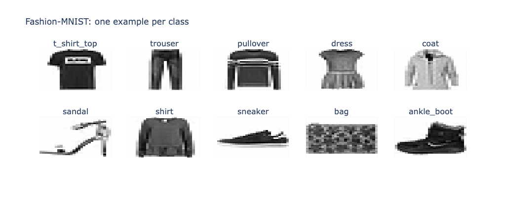
Figure 6-1. Fashion-MNIST Examples.
Building the Application
Prerequisites
You’ll need a Neo4j Aura free-tier instance with the connection details stored as environment variables.
Fashion-MNIST is fetched automatically via scikit-learn’s fetch_openml.
Loading the Data
We fetch Fashion-MNIST via scikit-learn, normalize and flatten the images, then build two DataFrames:
fashion = fetch_openml(name="Fashion-MNIST", version=1, as_frame=False)
X, y = fashion.data, fashion.target.astype(np.uint8)

train_images_raw = X[:60000].reshape(-1, 28, 28)
test_images_raw  = X[60000:].reshape(-1, 28, 28)

# Normalize to [0, 1] and flatten to 784-element vectors
train_images = (train_images_raw.astype("float32") / 255.0).reshape(-1, 784)
test_images  = (test_images_raw.astype("float32")  / 255.0).reshape(-1, 784)

train_df = pd.DataFrame({
    "id":     np.arange(len(train_images)),
    "vector": list(train_images),
    "label":  [CLASSES[l] for l in train_labels],
    "split":  "train"
})
Loading the Graph
We clear the database, create uniqueness constraints, load Category nodes for the 10 classes, then load Item nodes in batches of 500:
session.run("""
    CREATE CONSTRAINT category_name IF NOT EXISTS
    FOR (c:Category) REQUIRE c.name IS UNIQUE
""")
session.run("""
    CREATE CONSTRAINT item_uid IF NOT EXISTS
    FOR (i:Item) REQUIRE i.uid IS UNIQUE
""")

session.run("""
    UNWIND $names AS name
    MERGE (:Category {name: name})
""", names=CLASSES)
The uniqueness constraint is on uid, not id. Without it, items from different splits with the same integer id would conflict. The uid field – "train_0", "test_500" – is unique across the entire graph.
Items are loaded in chunks of 500 using UNWIND. Each item is linked to its category via BELONGS_TO:
session.run("""
    UNWIND $rows AS row
    CREATE (i:Item {
        uid:    row.uid,
        id:     row.id,
        label:  row.label,
        split:  row.split,
        vector: row.vector
    })
    WITH i, row
    MATCH (c:Category {name: row.label})
    CREATE (i)-[:BELONGS_TO]->(c)
""", rows=chunk)
With 70,000 items batched at 500, this is 140 transactions. Expect the full load to take several minutes on Aura’s free tier.
Creating the Vector Index
A single Cypher call creates the vector index using Euclidean distance:
session.run("""
    CREATE VECTOR INDEX item_vector IF NOT EXISTS
    FOR (i:Item) ON (i.vector)
    OPTIONS {indexConfig: {
        `vector.dimensions`: 784,
        `vector.similarity_function`: 'euclidean'
    }}
""")
Euclidean distance is appropriate for pixel vectors – it measures the total intensity difference across all 784 pixels. For semantic text embeddings, cosine similarity is usually the better choice.
t-SNE Visualization
Before querying the index, we use t-SNE to project the 784-dimensional vectors into 2D and verify that the categories form distinct clusters. We sample 60,000 training items and run t-SNE with the Barnes-Hut algorithm:
tsne = TSNE(
    n_components=2,
    random_state=42,
    method="barnes_hut",
    perplexity=30,
    max_iter=1000
)
X_tsne = tsne.fit_transform(train_images[:60000])
The resulting scatter plot, colored by class, shows clear clusters for most categories – trousers and bags are well separated; t-shirts, shirts and pullovers cluster more closely, which matches the visual similarity of those garments. This gives us confidence that the vector index will return meaningful nearest neighbors.
Figure 6-2 shows the result – most categories form distinct clusters, though t-shirt, shirt and pullover overlap, which matches their visual similarity.
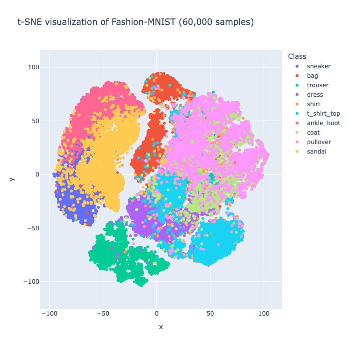
Figure 6-2. t-SNE Projection.
Query 1: k-NN Within the Training Set
The standard k-NN query fetches the query vector from Neo4j, then calls the vector index:
# Fetch the query vector
q = session.run("""
    MATCH (i:Item {id: $id, split: $split})
    RETURN i.vector AS vector, i.label AS label
""", id=QUERY_ID, split="train").single()

# k-NN search
result = session.run("""
    CALL db.index.vector.queryNodes('item_vector', $k, $vector)
    YIELD node AS i, score
    WHERE i.split = $split
    RETURN i.id AS id, i.label AS label, i.split AS split, score
    ORDER BY score DESC
""", k=K * 3, vector=q["vector"], split="train")
Two things to note. First, the score from Euclidean distance is inverted – a higher score means greater similarity (closer in vector space), not greater distance. Second, we fetch k * 3 candidates and filter to k after excluding the query item itself, which always appears in the results with a perfect score.
The image grid renders the query item and its nearest neighbors using Plotly’s go.Heatmap with colorscale="gray_r" – inverted grayscale gives white backgrounds with dark clothing outlines, which reads more naturally than the raw dark-background representation.
Query 2: k-NN Within the Test Set
The same pattern applied to a test-split query item. Because train and test items are in the same index, we filter by i.split = 'test' in the WHERE clause.
Query 3: Cross-Set Similarity Search
A train item queries against the test set, or vice versa. This tests whether the vector representations generalize across splits – whether a training image of a dress finds similar test images of dresses:
result = session.run("""
    CALL db.index.vector.queryNodes('item_vector', $k, $vector)
    YIELD node AS i, score
    WHERE i.split = 'test'
    RETURN i.id AS id, i.label AS label, i.split AS split, score
    ORDER BY score DESC
""", k=K * 3, vector=query_vector)
For most query items, the top test-set neighbors are in the same category as the query – the pixel vectors are consistent enough across the train/test split that cross-set search works reliably.
Query 4: Graph-Filtered k-NN
This is where the graph model adds value. We restrict the search to a specific category by traversing the BELONGS_TO relationship after the vector index call:
result = session.run("""
    CALL db.index.vector.queryNodes('item_vector', $k, $vector)
    YIELD node AS i, score
    MATCH (i)-[:BELONGS_TO]->(c:Category {name: $category})
    RETURN i.id AS id, i.label AS label, i.split AS split, score
    ORDER BY score DESC
""", k=K * 10, vector=query_vector, category="dress")
We fetch k * 10 candidates to ensure enough remain after the category filter. This is a post-filter pattern – the vector index finds the approximate nearest neighbors globally, then the graph traversal filters to the target category. For a balanced dataset like Fashion-MNIST, fetching 10x candidates is sufficient. For unbalanced categories a larger multiplier may be needed.
This pattern – vector search then graph filter – is the foundation of what chapter 7 builds into a full fraud detection system.
The Streamlit App
The app has a sidebar with controls for the query category, query split, results split filter, results category filter and k. A “Pick random item and search” button selects a random item from the chosen category and split, fetches its vector from Neo4j and runs the k-NN search.
The main area shows a summary of the query item and result count, an image grid of the query item and its nearest neighbors rendered as Plotly heatmaps, and a category breakdown bar chart showing which categories appear in the results. The image grid renders both the query image and result images from the in-memory Fashion-MNIST arrays rather than fetching pixel data from Neo4j – the vectors stored in Neo4j are the normalized float versions, not the original uint8 values needed for display.
Results persist in st.session_state across re-runs so the display doesn’t disappear when sidebar controls are adjusted.
What You’d Hit in Production
ANN vs exact search. Neo4j’s vector index uses approximate nearest neighbor search. For the Fashion-MNIST use case the approximation is excellent – the top-k results are indistinguishable from exact results in practice. For use cases where recall must be guaranteed (medical imaging, legal document retrieval), exact search may be required, which is slower but available.
Index creation time. Creating the vector index over 70,000 items with 784 dimensions takes a few minutes on Aura’s free tier. The index creation is asynchronous – check the index state before querying.
Post-filter overhead. The graph-filtered k-NN query (Query 4) fetches k * 10 candidates to ensure enough survive the category filter. If the target category is rare in the index, you may need a larger multiplier. An alternative is pre-filtering – restricting the index scan to nodes of the target category – but this isn’t supported in Neo4j’s current vector index implementation.
Vector storage. Each 784-element float32 vector takes around 3KB of storage. 70,000 vectors takes around 200MB, which is within Aura’s free-tier limit but leaves little headroom. For higher-dimensional vectors – 384-element sentence embeddings, 1536-element OpenAI embeddings – storage requirements grow accordingly.
The split filter. The WHERE i.split = $split clause in queries 1 and 2 runs after the ANN index returns candidates. It’s a post-filter, not a pre-filter. For very unbalanced splits, fetch more candidates than you need.
Going Further
Vector search finds similar items by distance in vector space. Graph traversal finds connected items by relationship. In this chapter we combined them: a vector search followed by a graph filter in a single Cypher statement. That combination is powerful, but both steps still ran independently – the vector search found candidates globally, then the graph reduced them.
Chapter 7 inverts the order and tightens the integration. We use vector search to find semantically suspicious transactions, then use graph traversal to confirm whether those transactions form a circular money flow – a fraud ring. The vector component identifies candidates the graph component couldn’t find alone; the graph component validates structure the vector component can’t see. That’s the full combination, and it’s where this book ends up.
Chapter 7: Graph + Vector
What Is It?
Vector search answers “which transactions look suspicious?” Graph traversal answers “which accounts are connected through circular money flows?” Used together, they answer a third question that neither can answer alone: “which suspicious-looking transactions are part of a coordinated fraud ring?”
This is the combination the book has been building toward. Every capability in the preceding chapters – graph traversal, full-text search, geospatial queries, temporal reasoning, document properties, vector search – was a standalone tool. Chapter 7 brings two of the most powerful together in a single Cypher query: a vector similarity search that identifies semantically suspicious transactions, followed immediately by a graph traversal that checks whether those transactions form a circular ring pattern.
The result is a fraud detection system with three operational modes. Pure graph ring detection finds coordinated circular money flows using Cypher pattern matching. Pure vector search finds transactions whose prose descriptions resemble known fraud language. Graph + vector combined does both in a single query, surfacing only those suspicious transactions that also participate in a ring – a much stronger fraud signal than either approach alone.
When Would You Reach for It?
The graph + vector combination earns its place when your fraud signal has two components: semantic content (what a transaction is described as) and structural position (who sent it and to whom, and how those accounts are connected). Either component alone produces noise. Together they produce signal.
Reach for this pattern when:
- You have text or embeddings that can identify suspicious entities
- You have a graph that can validate whether those entities are structurally connected in a suspicious pattern
- You need to run both in a single query rather than two separate systems
- The false positive rate from either approach alone is too high for the use case
Financial fraud is the canonical application, but the same pattern applies to social network abuse detection, supply chain anomaly detection and any domain where suspicious behavior has both a semantic signature and a structural pattern.
The Use Case
We build a synthetic fraud detection system with 1,000 bank accounts and approximately 50,000 transactions. The vast majority of transactions are legitimate – ring transactions account for less than 0.3% of the data, mirroring real-world fraud rates. Hidden in the transaction graph are planted fraud rings of 3, 4 and 5 hops, each with amounts tightly clustered between $2,000 and $9,999 and each completing within 90 minutes.
The challenge is finding those rings without knowing in advance which accounts or transactions are involved.
The Data
The dataset is generated entirely in the notebook with a fixed random seed for reproducibility.
Accounts: 1,000 nodes with account_id, customer_name and risk_score properties. About 20% of account names are business names (LLC, Inc, Corp); the rest are personal names.
Transactions: ~50,000 total. Each has tx_id, amount, timestamp, is_fraud_ring (the hidden ground truth), description (a prose sentence) and embedding (a 384-element fastembed vector).
Fraud rings: planted in three sizes – five 3-hop rings (min amount $4,000), five 4-hop rings (min amount $3,500) and three 5-hop rings (min amount $3,000). Twenty additional random noise rings of 3-6 hops add realistic background complexity. Ring transactions are spaced 3-15 minutes apart within each ring, so the full ring completes within 90 minutes.
Transaction descriptions: ring transactions use templates that sound like structuring or layering: “Structured transfer of $X through intermediary account – round-trip pattern.” Legitimate transactions describe plausible purchases at fictional merchants.
The graph model is:
(:Account {account_id, customer_name, risk_score})
  -[:MADE]->
(:Transaction {tx_id, amount, timestamp, is_fraud_ring, description, embedding})
  -[:TO]->
(:Account)
Building the Application
Prerequisites
You’ll need a Neo4j Aura free-tier instance with the connection details stored as environment variables.
This chapter uses fastembed for embedding the transaction descriptions. fastembed downloads the BAAI/bge-small-en-v1.5 model (~23 MB) on first use and caches it locally. The model produces 384-dimensional embeddings and runs entirely locally – no API key required.
Loading the Embedding Model
from fastembed import TextEmbedding

embed_model = TextEmbedding("BAAI/bge-small-en-v1.5")

def get_embedding(text: str) -> list:
    return list(embed_model.embed([text]))[0].tolist()

EMBEDDING_DIMS = len(get_embedding("test"))  # 384
We call embed_model.embed([text]) with a list and take the first result. This is slightly less efficient than batch embedding but keeps the helper function simple. For the full 50,000 transactions we embed in batches.
Loading the Graph
We load accounts first, then embed and load transactions in batches of 500. The embedding step takes a few minutes for 50,000 transactions:
def embed_and_load_batch(session, batch):
    texts  = [r["description"] for r in batch]
    embeds = list(embed_model.embed(texts))
    rows   = [
        {**rec, "embedding": embeds[i].tolist()}
        for i, rec in enumerate(batch)
    ]
    session.run("""
        UNWIND $rows AS row
        MATCH (src:Account {account_id: row.source_id})
        MATCH (tgt:Account {account_id: row.target_id})
        CREATE (t:Transaction {
            tx_id:         row.tx_id,
            amount:        row.amount,
            timestamp:     row.timestamp,
            is_fraud_ring: row.is_fraud_ring,
            description:   row.description,
            embedding:     row.embedding
        })
        CREATE (src)-[:MADE]->(t)
        CREATE (t)-[:TO]->(tgt)
    """, rows=rows)
Each transaction is connected to two accounts: the source account via MADE and the target account via TO. This two-relationship pattern is what enables Cypher to traverse ring patterns using comma-separated MATCH clauses.
Creating the Vector Index
The vector index uses cosine similarity, which is appropriate for sentence embeddings:
session.run(f"""
    CREATE VECTOR INDEX transaction_embeddings
    FOR (t:Transaction) ON (t.embedding)
    OPTIONS {{indexConfig: {{
        `vector.dimensions`: {EMBEDDING_DIMS},
        `vector.similarity_function`: 'cosine'
    }}}}
""")
We poll until the index is ONLINE before running any similarity queries – index creation is asynchronous.
Query 1: Pure Graph Ring Detection
Cypher expresses a 3-hop ring as a comma-separated pattern that returns to its origin:
result = session.run("""
    MATCH (a1:Account)-[:MADE]->(t1:Transaction)-[:TO]->(a2:Account),
          (a2)-[:MADE]->(t2:Transaction)-[:TO]->(a3:Account),
          (a3)-[:MADE]->(t3:Transaction)-[:TO]->(a1)
    WHERE t1.amount >= $min_amount AND t1.amount <= $max_amount
      AND t2.amount >= $min_amount AND t2.amount <= $max_amount
      AND t3.amount >= $min_amount AND t3.amount <= $max_amount
      AND a1.account_id < a2.account_id
      AND a1.account_id < a3.account_id
      AND abs(duration.between(datetime(t1.timestamp),
              datetime(t2.timestamp)).minutes) < 90
      AND abs(duration.between(datetime(t2.timestamp),
              datetime(t3.timestamp)).minutes) < 90
    RETURN a1.account_id AS account_1,
           a2.account_id AS account_2,
           a3.account_id AS account_3,
           t1.amount AS amount_1,
           t2.amount AS amount_2,
           t3.amount AS amount_3
    LIMIT $limit
""", min_amount=min_amount, max_amount=max_amount, limit=limit)
Three filters work together to eliminate coincidental rings:
Amount range (min_amount to max_amount=9999): legitimate transactions go up to $50,000. Ring transactions are generated between $2,000 and $9,999. The upper bound eliminates the vast majority of coincidental cycles formed by legitimate high-value transactions.
Timestamp constraint (within 90 minutes): ring hops are spaced 3-15 minutes apart, so a 3-hop ring completes in at most 30 minutes. A 90-minute window catches all planted rings while eliminating coincidental cycles between transactions days apart.
Deduplication (a1.account_id < a2.account_id AND a1.account_id < a3.account_id): without this, every ring appears multiple times – once for each starting account. The alphabetic ordering constraint ensures each ring is returned exactly once.
One critical Cypher detail: the ring pattern uses comma-separated MATCH clauses, not juxtaposed patterns. Juxtaposing the patterns – writing them one after another without a comma – causes a syntax error in Neo4j 5.x. The comma is required.
The same structure extends naturally for 4-hop and 5-hop rings by adding one more account and transaction to the pattern. The equivalent SQL requires a completely rewritten recursive CTE for each additional hop.
Query 2: Pure Vector Search
Pure vector search embeds the query string and finds semantically similar transactions:
query_embedding = get_embedding("circular money transfer through intermediary accounts")

result = session.run("""
    CALL db.index.vector.queryNodes(
        'transaction_embeddings', $top_k, $embedding
    ) YIELD node AS t, score
    MATCH (src:Account)-[:MADE]->(t)-[:TO]->(tgt:Account)
    RETURN t.tx_id         AS tx_id,
           src.account_id  AS source_account,
           tgt.account_id  AS target_account,
           t.amount        AS amount,
           t.is_fraud_ring AS is_fraud_ring,
           t.description   AS description,
           score
    ORDER BY score DESC
""", embedding=query_embedding, top_k=top_k)
The vector search returns transactions whose descriptions are semantically similar to the query. Because ring transactions were generated with structuring and layering language, queries about circular money movement consistently return ring transactions with cosine similarity scores above 0.90. But pure vector search has no awareness of whether those transactions form rings – it can flag individual suspicious transactions without confirming the pattern.
Query 3: Graph + Vector Combined
The combined query runs vector search first, then immediately extends into graph traversal in the same Cypher statement:
result = session.run(f"""
    // Step 1: vector search finds semantically suspicious transactions
    CALL db.index.vector.queryNodes(
        'transaction_embeddings', $top_k, $embedding
    ) YIELD node AS t, score
    WHERE score >= $threshold

    // Step 2: get the source account of each suspicious transaction
    MATCH (a1:Account)-[:MADE]->(t)

    // Step 3: check if the target account is part of a ring
    {ring_match}
    WHERE {ring_where}

    RETURN DISTINCT
        t.tx_id         AS tx_id,
        score           AS similarity,
        a1.account_id   AS entry_account,
        t.amount        AS entry_amount,
        t.is_fraud_ring AS is_fraud_ring,
        {ring_return}
    ORDER BY score DESC
""", embedding=query_embedding, top_k=top_k, threshold=threshold,
     min_amount=min_amount, max_amount=max_amount)
The ring_match and ring_where strings are built dynamically based on the ring_hops parameter (3 or 4). For a 3-hop ring check, ring_match follows the target account through three MADE/TO hops back to itself; ring_where applies the amount and timestamp filters to those ring transactions; ring_return returns the list of ring account IDs.
This is the key result: only transactions that are both semantically suspicious (high cosine similarity to the query) and structurally connected (part of a circular ring pattern) appear in the output. The is_fraud_ring flag confirms against the hidden ground truth.
Ring Summary
A batch ring summary query counts all detected rings and confirmed fraud:
result = session.run("""
    MATCH (a1:Account)-[:MADE]->(t1:Transaction)-[:TO]->(a2:Account),
          (a2)-[:MADE]->(t2:Transaction)-[:TO]->(a3:Account),
          (a3)-[:MADE]->(t3:Transaction)-[:TO]->(a1)
    WHERE t1.amount >= 2000 AND t1.amount <= 9999
      AND t2.amount >= 2000 AND t2.amount <= 9999
      AND t3.amount >= 2000 AND t3.amount <= 9999
      AND a1.account_id < a2.account_id
      AND a1.account_id < a3.account_id
      AND abs(duration.between(datetime(t1.timestamp),
              datetime(t2.timestamp)).minutes) < 90
      AND abs(duration.between(datetime(t2.timestamp),
              datetime(t3.timestamp)).minutes) < 90
    RETURN count(*) AS ring_count,
           round(avg(t1.amount + t2.amount + t3.amount), 2) AS avg_total_amount,
           sum(CASE WHEN t1.is_fraud_ring = true THEN 1 ELSE 0 END) AS confirmed_fraud
""")
With the amount range and timestamp filters applied, this query returns 13 detected rings, all 13 confirmed as planted fraud – 100% precision. The ring summary is a full graph scan and runs slowly; it’s designed as a batch analytical query, not an interactive one.
Ring Visualization
Detected rings are visualized as a NetworkX force-directed graph rendered with Plotly. Red nodes (#E63946) represent accounts; grey edges show the direction of money flow. The spring layout with k=1.0 spreads the nodes organically without forcing rigid geometric shapes:
G = nx.DiGraph()
for r in ring_records:
    ring_nodes = [r[f"account_{i}"] for i in range(1, hops + 1)]
    for i, node in enumerate(ring_nodes):
        G.add_node(node)
        G.add_edge(node, ring_nodes[(i + 1) % hops], amount=r[f"amount_{i+1}"])

pos = nx.spring_layout(G, seed=RANDOM_SEED, k=1.0, iterations=100)
Figure 7-1 shows the detected 3-hop rings – each cluster of three nodes forms a circular money flow.
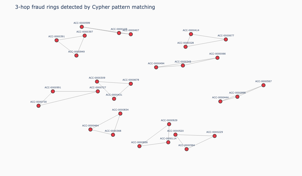
Figure 7-1. 3-hop Fraud Rings.
The Streamlit App
The sidebar has a query type selector – Pure Graph, Pure Vector, Graph + Vector – with parameters that adapt to the selection. Pure Graph exposes hop count (3, 4 or 5), min/max amount and a result limit. Pure Vector exposes a query text area, vector candidate count and similarity threshold. Graph + Vector exposes all of the above.
The app has two tabs. The Query Explorer tab runs the selected query and displays results as a dataframe – ring paths and amounts for pure graph, transaction details and fraud flags for pure vector and entry transaction plus ring structure for graph + vector. The Ring Visualization tab is active after a Pure Graph query and renders the spring-layout ring graph.
All results persist in st.session_state across re-runs. The embedding model is cached with @st.cache_resource so it loads once and stays in memory for the session – fastembed downloads are slow on first run but instant on subsequent ones.
What You’d Hit in Production
Embedding throughput. fastembed with BAAI/bge-small-en-v1.5 runs on CPU and embeds roughly 500-1,000 short sentences per second on a modern machine. For 50,000 transactions this takes a few minutes. For millions of transactions at ingestion time, batch embedding with a GPU or a hosted embedding API would be significantly faster.
The query parameter conflict. The Neo4j Python driver reserves query as a keyword argument for the Cypher string itself. Never use query as a parameter name in your Cypher parameters. Use search_query, embedding, q or any other name. This applies everywhere in the codebase, not just chapter 7.
Ring summary performance. The ring summary query scans the full transaction graph. On 50,000 transactions it takes 10-30 seconds. For production workloads you’d run this as a scheduled batch job rather than on demand, and consider creating additional indexes to speed up the traversal.
The max_amount filter. Without the upper-bound amount filter (amount <= 9999), legitimate transactions with amounts up to $50,000 form thousands of coincidental 3-hop cycles. The amount ceiling is not an arbitrary threshold – it’s grounded in the dataset design. In a real system you’d tune this threshold empirically based on the known amount distribution of your fraud cases.
Comma-separated MATCH patterns. Neo4j 5.x requires comma-separated MATCH clauses for multi-hop ring patterns. Juxtaposed patterns – written one after another without a comma – cause a syntax error.
Going Further
This chapter closes the arc the book has been tracing. We started with the graph model in chapter 1 – stations, connections, traversal. We added capability by capability: text search, spatial queries, temporal data, document properties, vector similarity. Chapter 7 combines the last two into something that neither graph databases nor vector databases can do alone in a single query.
The fraud detection system in this chapter is a demonstration, not a production deployment. A real system would need continuous ingestion, a real-time embedding pipeline, alerting thresholds calibrated against labeled historical data and human review of flagged cases. But the core pattern – vector search to identify candidates, graph traversal to validate structure – is the right architecture for this class of problem, and Neo4j is the right database to run it on.
That’s Neo4j beyond the graph.
Conclusions
What We Built
Over seven chapters we built seven example applications, each demonstrating a different Neo4j capability. We found shortest paths on the London Underground, discovered research papers through full-text search, queried air quality data across the Pyrenees corridor, analyzed five years of S&P 500 prices, managed a library inventory with heterogeneous metadata, searched 70,000 fashion images by visual similarity and detected fraud rings by combining vector search with graph traversal.
Every notebook runs on Neo4j Aura’s free tier. Every application is a working Streamlit app. The gotchas are real. The “what you’d hit in production” sections are meant.
What We Learned
Neo4j is more than a graph database
The most consistent theme across the seven chapters is that Neo4j’s graph model is the foundation, not the ceiling. Full-text search, geospatial indexing, temporal queries, document-style properties and vector similarity are all native capabilities – not integrations with external systems, not add-ons that require separate infrastructure. They work with Cypher and they work together.
Many Neo4j users never explore beyond the graph. The chapters in this book are an attempt to show what’s available when you do.
The combination is the point
Each capability is useful on its own. But the most compelling demonstrations in this book are the ones where two capabilities work together: a spatial proximity query that uses a pre-computed graph for cross-border neighbor lookups, a full-text search that extends into citation traversal, a vector search that filters by graph structure in a single Cypher statement.
Chapter 7 is the clearest example. Pure vector search flags suspicious transactions. Pure graph search finds circular money flows. Neither alone is enough – the combination, in a single query, is what produces a strong fraud signal. That combination is something no relational database, document database or standalone vector database can replicate naturally.
Cypher is expressive enough
One thing that might surprise readers coming from SQL is how much Cypher can do in a single statement. The ring detection query in chapter 7 – vector search, source account lookup, three-hop ring traversal, amount and timestamp filters, deduplication, all in one query – would be a multi-step process in any other system. The fact that it’s a single Cypher statement isn’t a novelty. It’s what makes the pattern operationally practical.
The “when to look elsewhere” sections are also true
Neo4j is not the right tool for every problem in this book. High-frequency time series data belongs in a purpose-built time series database. Pure geospatial problems belong in a GIS platform. Billions of documents with no graph component belong in a dedicated search engine. Adding Neo4j to a stack that doesn’t need its graph or multi-model capabilities means unnecessary complexity.
The right question is not “can Neo4j do this?” – it usually can. The right question is “does the graph or multi-model dimension add enough value to justify Neo4j over a simpler alternative?”
A Practical Decision Guide
Use Neo4j’s native graph model when the connections between entities are the signal: transport networks, social graphs, supply chains, recommendation engines, fraud detection based on account relationships.
Add full-text search when your graph nodes carry text and you want to combine keyword or phrase search with graph traversal in a single query.
Add geospatial when your entities have coordinates and meaningful relationships to each other and you want to query both dimensions together.
Add temporal when time-varying data are connected to other entities in a graph and you want to combine date-range queries with traversal.
Add document-style properties when your nodes carry variable-structure metadata that doesn’t need to be independently indexed or traversed as graph structure. Serialize as JSON, parse with APOC. Promote frequently filtered fields to top-level properties.
Add vector search when similarity is the query – finding items that resemble a given item, regardless of shared property values. Combine with graph filters when the interesting constraint is structural, not just categorical.
Combine graph and vector when suspicious behavior has both a semantic signature and a structural pattern. Vector search to identify candidates. Graph traversal to validate structure. The combination, in a single Cypher query, is Neo4j’s most distinctive capability.
The table below summarizes the specific Neo4j features and functions used in each chapter. It serves as a quick reference for the capabilities covered in this book.
| Chapter | Capability | Key Features |
|---|---|---|
| 1 | Native Graph | Node and relationship storage, bidirectional relationships, shortestPath(), variable-depth traversal (*1..n), UNWIND batch operations, uniqueness constraints |
| 2 | Full-Text Search | Apache Lucene integration, BM25 relevance scoring, keyword/phrase/fuzzy (~) search, FULLTEXT INDEX, db.index.fulltext.queryNodes(), asynchronous index polling |
| 3 | Geospatial | Native point type, POINT INDEX, point.distance(), composite uniqueness constraints, elementId() deduplication, latest-record pattern with collect()[0] |
| 4 | Temporal | Native date and datetime types, range index on date properties, date() filtering, min()/max() date anchoring |
| 5 | Document-Style Properties | JSON string property storage, apoc.convert.fromJsonMap(), apoc.convert.toJson(), apoc.map.removeKey(), ANY() over deserialized lists, map spread operator |
| 6 | Vector Search | VECTOR INDEX, ANN search, euclidean similarity, db.index.vector.queryNodes(), post-filter oversampling (k * n), graph-filtered k-NN |
| 7 | Graph + Vector | Vector search + graph traversal in a single Cypher query, comma-separated MATCH for ring detection, duration.between() timestamp constraints, dynamic hop count, DISTINCT deduplication |
What Comes Next
The multi-model database landscape is moving quickly. Neo4j continues to expand product capabilities. APOC continues to grow. The Graph Data Science library adds community detection, centrality algorithms and machine learning pipelines that build directly on the graph model.
The specific procedures and syntax in this book may evolve. The underlying capabilities – and the architectural patterns that make them useful – will not.
A Final Note
The goal of this book was not to argue that Neo4j should replace every database in your stack. It was to show that if you’re using Neo4j or considering it for a graph use case, you already have access to full-text search, geospatial queries, temporal reasoning, document properties and vector similarity. Combining these capabilities with graph traversal is something no other database does as naturally.
This book is supported with Jupyter notebooks and Streamlit applications. The best way to decide whether any of these capabilities fits your use case is to run the code.
Free Books
The SingleStore Cookbook: Recipes for Multi-Model, Machine Learning and AI Data Engineering
A hands-on cookbook covering SingleStore’s multi-model capabilities, from time series and geospatial data through vector search, machine learning pipelines and AI-powered applications. The recipes draw on first-hand experience building applications with the platform and are organized into four parts:
- Multi-Model
- Streaming and Big Data Pipelines
- Machine Learning
- AI and Agentic Frameworks
Seven Vector Databases in Seven Days
A practical guide that takes one vector database per day and pairs each with a use case chosen to showcase that database’s strengths. Databases covered:
- PostgreSQL and pgvector - Semantic job search
- MongoDB Atlas - Recipe finder
- Pinecone - E-commerce search
- Weaviate - Research paper discovery
- Neo4j - Fraud detection
- Snowflake - Customer support analytics
- Databricks - RAG over internal documents
Each chapter is self-contained, comes with a Jupyter notebook and gives an assessment of when you’d look elsewhere.
Generative AI: A Manager’s Guide

A practical guide for managers, directors and executives who need to make decisions about AI in their organizations, not the engineers building it, but the people responsible for making it work well. The book uses a single central metaphor, the Digital Intern, to frame what AI is genuinely good at, where it falls short and what managing it actually requires. It covers governance, risk, board-level accountability, business case building and the organizational change of moving from pilot to embedded capability.
Seven Ways to Do Vector Search in Python
A practitioner’s guide that benchmarks seven Python libraries against the same dataset, measuring recall and latency consistently so you can compare like-for-like. Libraries covered:
- FAISS
- Voyager
- Scikit-learn NearestNeighbors
- PyNNDescent
- USearch
- Chroma
- LanceDB
Each chapter covers one library, explains what it’s genuinely good at and when you’d reach for something else.
Real-Time Vehicle Tracking with Neo4j, Databricks Lakebase and OpenStreetMap
A fleet operations demo that puts ten simulated vehicles onto real road networks loaded from OpenStreetMap. The architecture:
- Neo4j Aura holds the road network graph
- Databricks Lakebase stores live vehicle positions
- Databricks Lakehouse handles historical analytics
Two Streamlit dashboards display live positions and trend data. The primary demo uses the London Borough of Merton, with additional configurations for San Francisco and Singapore.
Real-Time Supply Chain Routing with Neo4j, Snowflake Postgres and Confluent Kafka
A supply chain routing demo that combines graph-based route optimization with real-time event streaming. The architecture:
- Neo4j Aura holds the supplier and logistics network graph
- Snowflake Postgres stores product and inventory data
- Confluent Kafka streams supply chain events in real time
Route queries traverse the graph to find optimal paths between suppliers, warehouses and distribution centers under live capacity and disruption constraints.
Neo4j Beyond the Graph
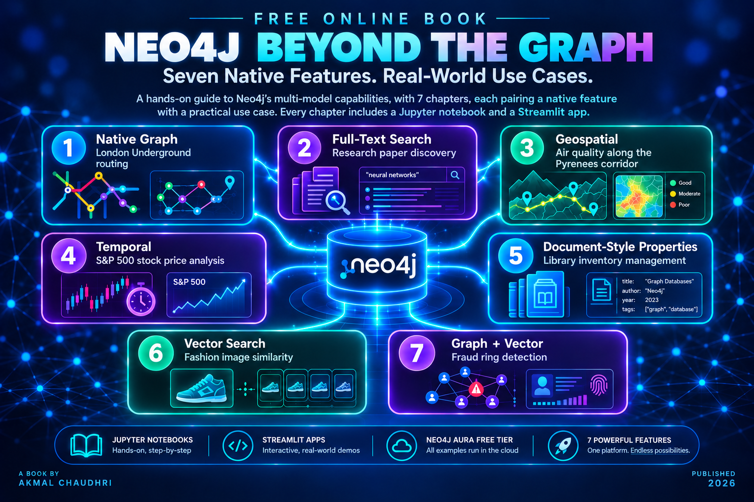
A hands-on guide to Neo4j’s multi-model capabilities, going beyond graph traversal to explore seven native features of the platform. Each chapter pairs one capability with a use case chosen to showcase it:
- Native Graph - London Underground routing
- Full-Text Search - Research paper discovery
- Geospatial - Air quality along the Pyrenees corridor
- Temporal - S&P 500 stock price analysis
- Document-Style Properties - Library inventory management
- Vector Search - Fashion image similarity
- Graph + Vector - Fraud ring detection
Every chapter comes with a Jupyter notebook and a Streamlit application. All examples run on Neo4j Aura’s free tier.
Seven Ways to Use Jev

A practical guide to TypeSafe AI’s structured decision model, exploring seven domains where a single Choice call – structured state in, typed decision out, calibrated confidence alongside – replaces brittle rules-based logic. Each chapter pairs one domain with a hands-on Jupyter notebook and examines what the confidence score reveals about the decision:
- Transit Routing - Northern Line branch triage using a NetworkX graph
- Customer Support Triage - Ticket routing by team and priority
- Financial Fraud Detection - Flag or pass with a three-tier confidence response
- Content Moderation - Approve, flag or remove user-generated content
- Supply Chain Disruption - Alternative supplier selection under live constraints
- Hiring Screening - CV screening against a structured job description
- Medical Symptom Triage - Care pathway assignment with a conservative bias
A recurring theme across all seven chapters: the confidence score is more informative than the decision itself for uncertain cases and the threshold between automatic routing and human review is always a business decision, not a technical one.
Lessons Learned Putting Jev Inside Neo4j
A hands-on account of building a Neo4j function and batch procedure in Java that ask a model to make a decision about a node and store the answer back in the graph. The book follows one running example, 500 synthetic transactions and each chapter adds the code that the previous chapter’s problem called for. The lessons:
- Why in the Database - Where a decision belongs and what the finished function returns
- A First Working Function - Converting Neo4j’s types on the way in and out
- Failures as Data - Returning errors as values so one bad node can’t stop a query
- Testing Without a Network - Seams for the network and the clock, with 68 fast tests
- Keeping the Key Safe - Sending a credential only to the host the parser reports
- Many at Once - A bounded, ordered pool and a measured concurrency sweep
- Running It Locally - Swapping in a small local model and seeing how the judgment changes
Every chapter with code has its own folder in the repository and each Cypher script also comes as a notebook, so you can use whichever you prefer. The results are reported as measured, including the ones we can’t explain!